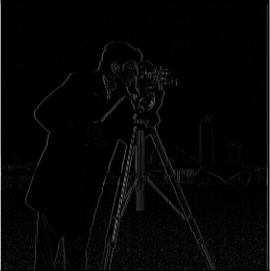
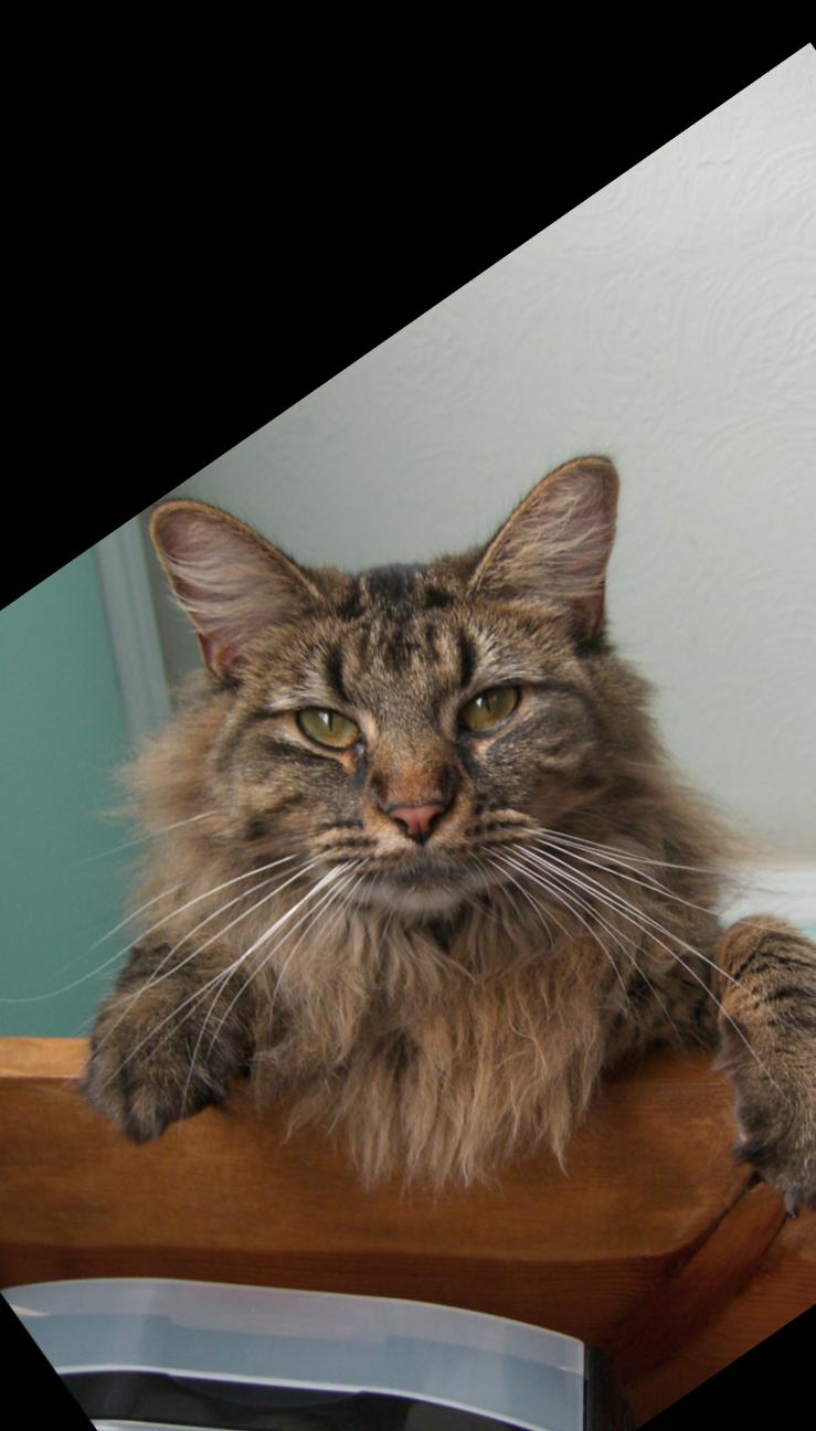
Sometimes, it is useful to find the edges of an image. There are lots of way to do this, and we will explore the approach using finite difference operator.
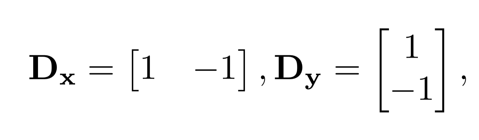
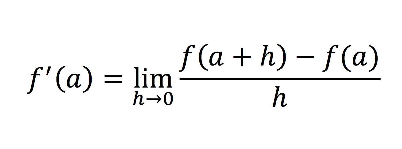
This is the simplest filters we can use to get the derivatives of the images. You might think this looks familiar to an equation in high school , and you are correct. We can think of this filter as the follow:
In the discretized scenario such as image, we would naturally choose the adjacent pixel as the smallest possible step (h) you could take, thus we have the finite filter.
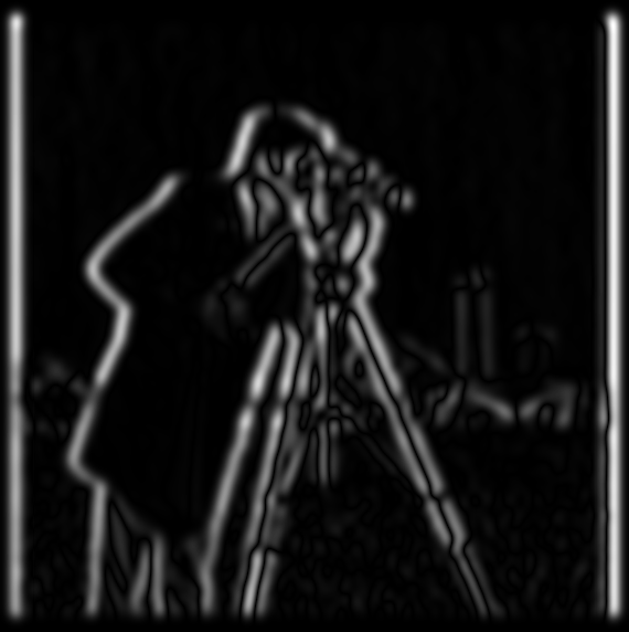
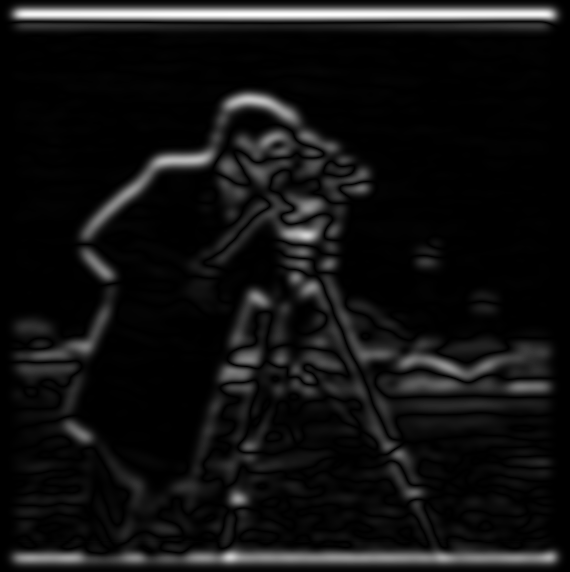
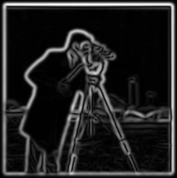
Below are the result.
|
|
|
|
|
|
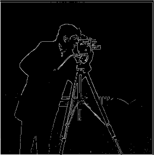
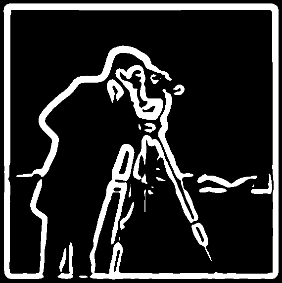
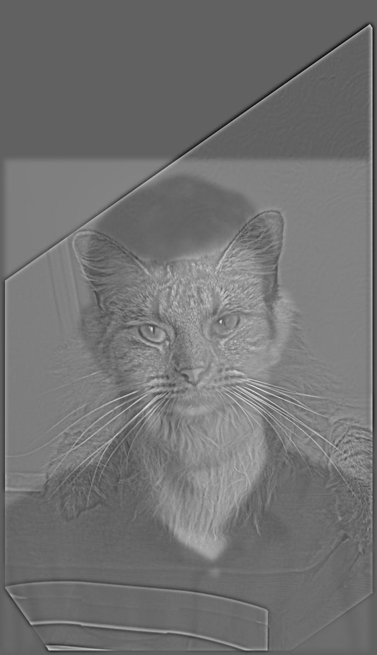
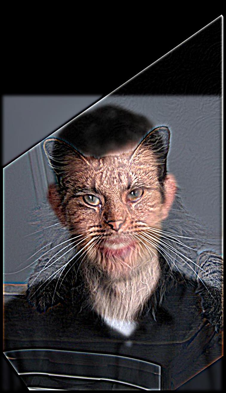
One important thing to note here is that the picked threshold has a huge impact on the binarized image. As you can see in the last image, the background is gone, and this is because we don't want to include both noise and background in the final image, so we have to tradeoff detail with noise.
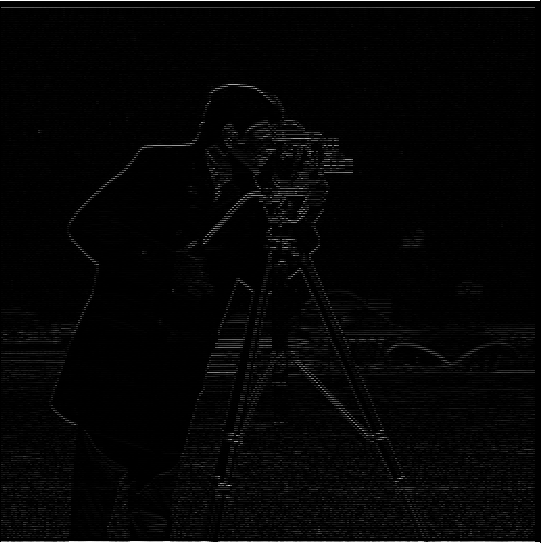
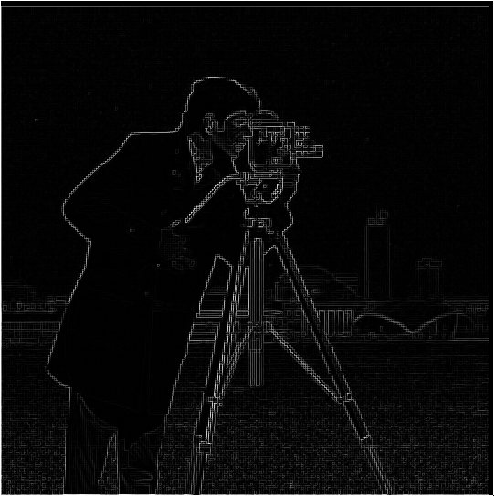
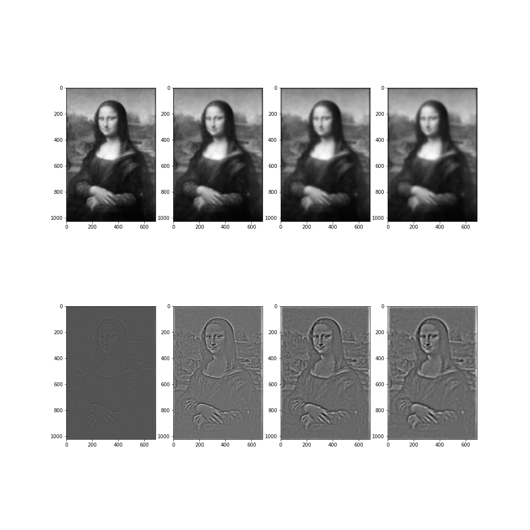
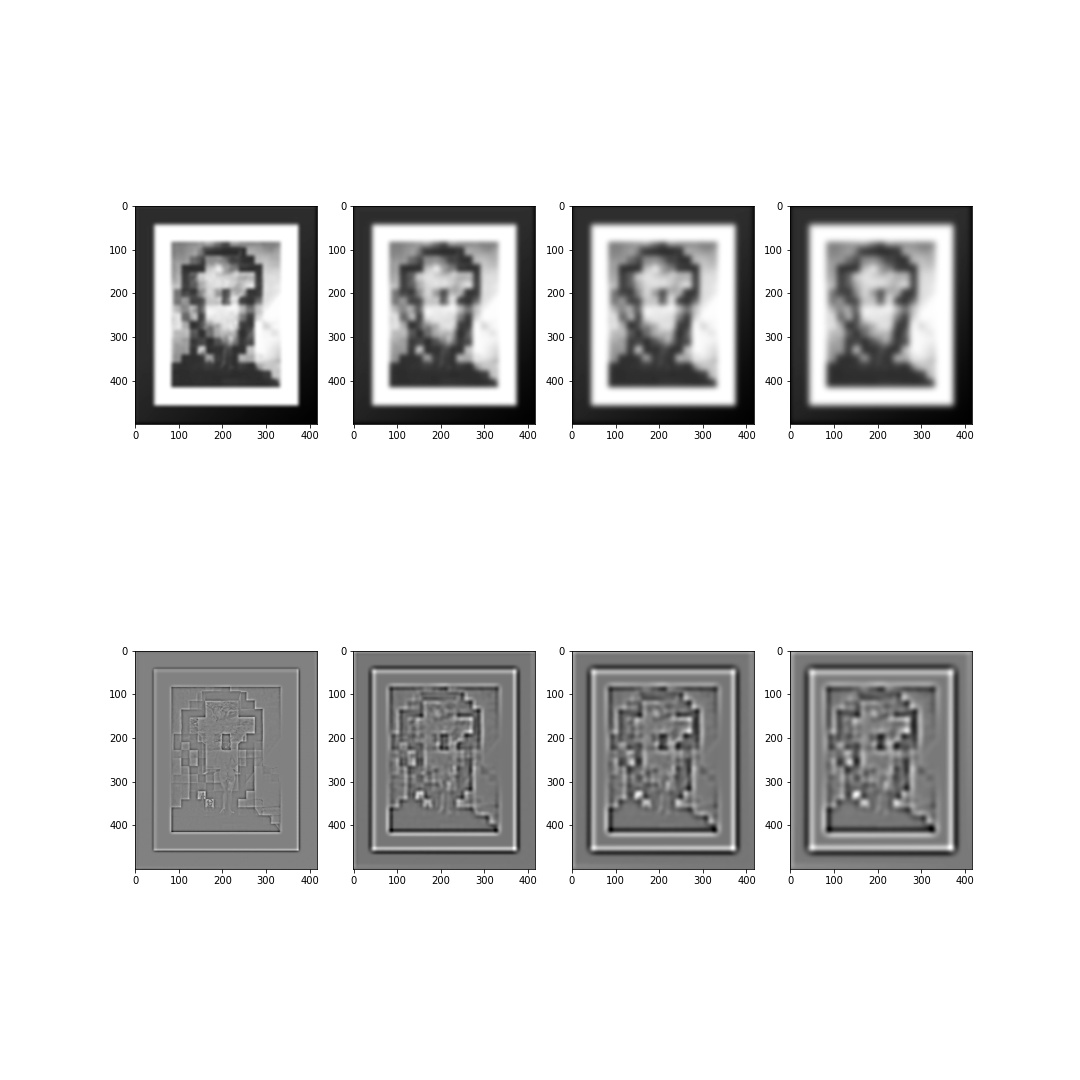
In practice, finite difference operator is not ideal because of its high frequency noise. As we know the noise can be reduced by simply blurring the image, gaussian filter can be convolved with the image to get a better result.
|
|
|
|
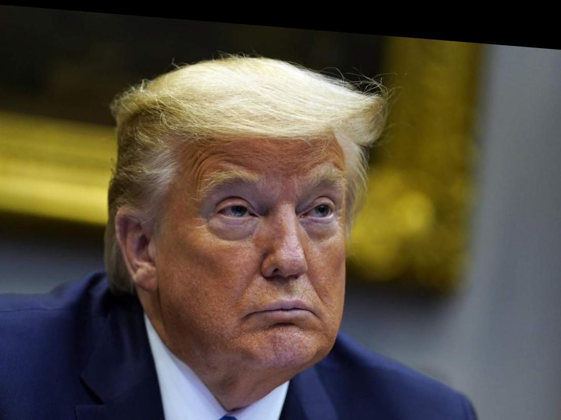
The above is the result of running part 1 with a blurred image. As expected, the high frequency element (edge) is flattened out, and we can even retrieve part of the background which we can't in part 1; however, the trade off is the loss of details in important part of the image such as the man's face.

|

|
To accelerate the process, we can first convolve the finite filters with the gaussian filter so that we don't have to convolve twice.

|
|
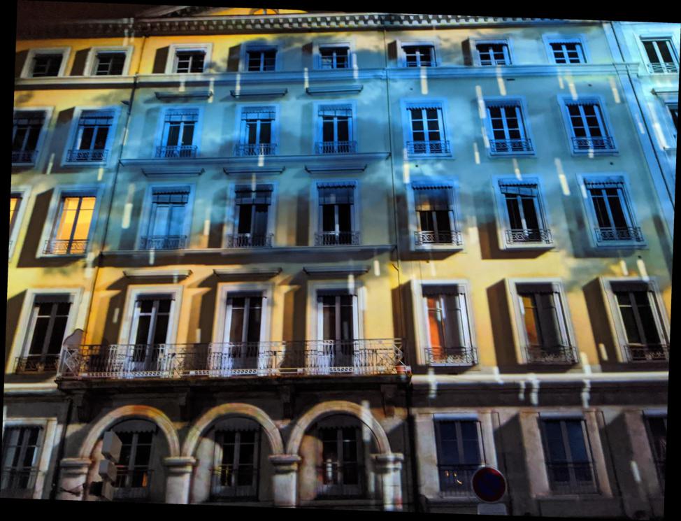
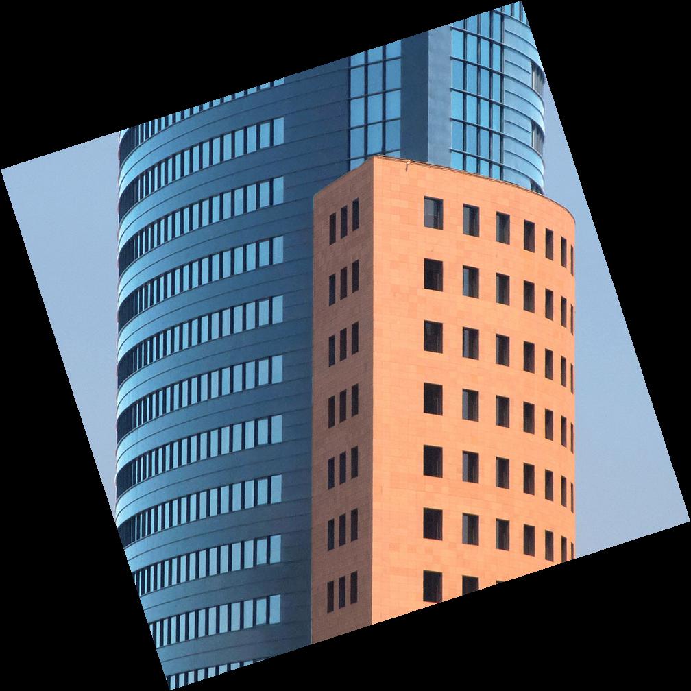
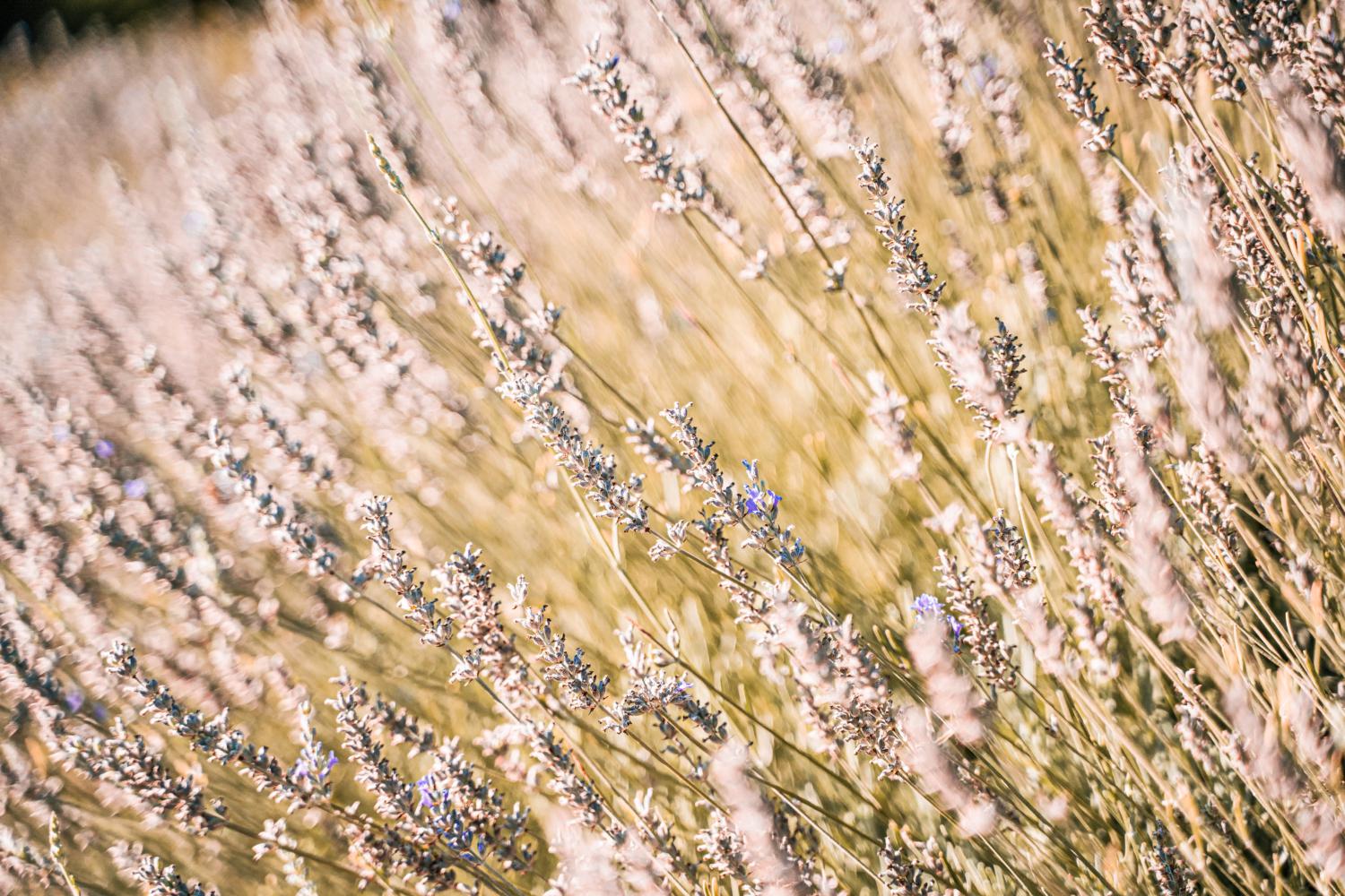
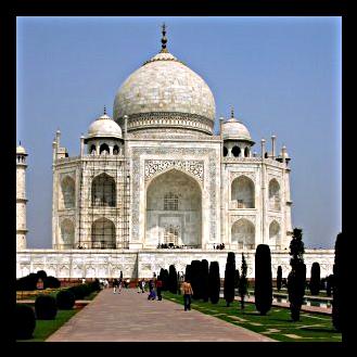
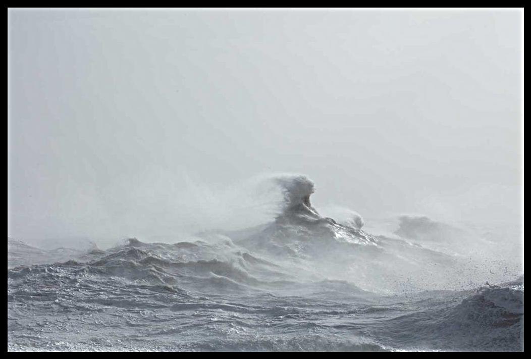
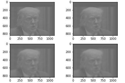
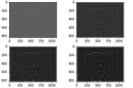
Sometimes, images that you have taken are not perfect. It is possible to have problems like motion blur, tilted image, etc. Here, we will help you to straighten the image again so you can show off your beautiful image in the correct perspective. What we have learnt so far is the finite filters and its capability to calculate gradient of the image. Interestingly, we can use the x and y gradient to calculate the angle of the edge to perform straightening. Equation is shown below.
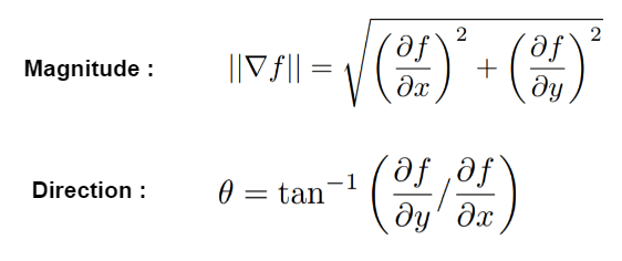
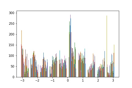
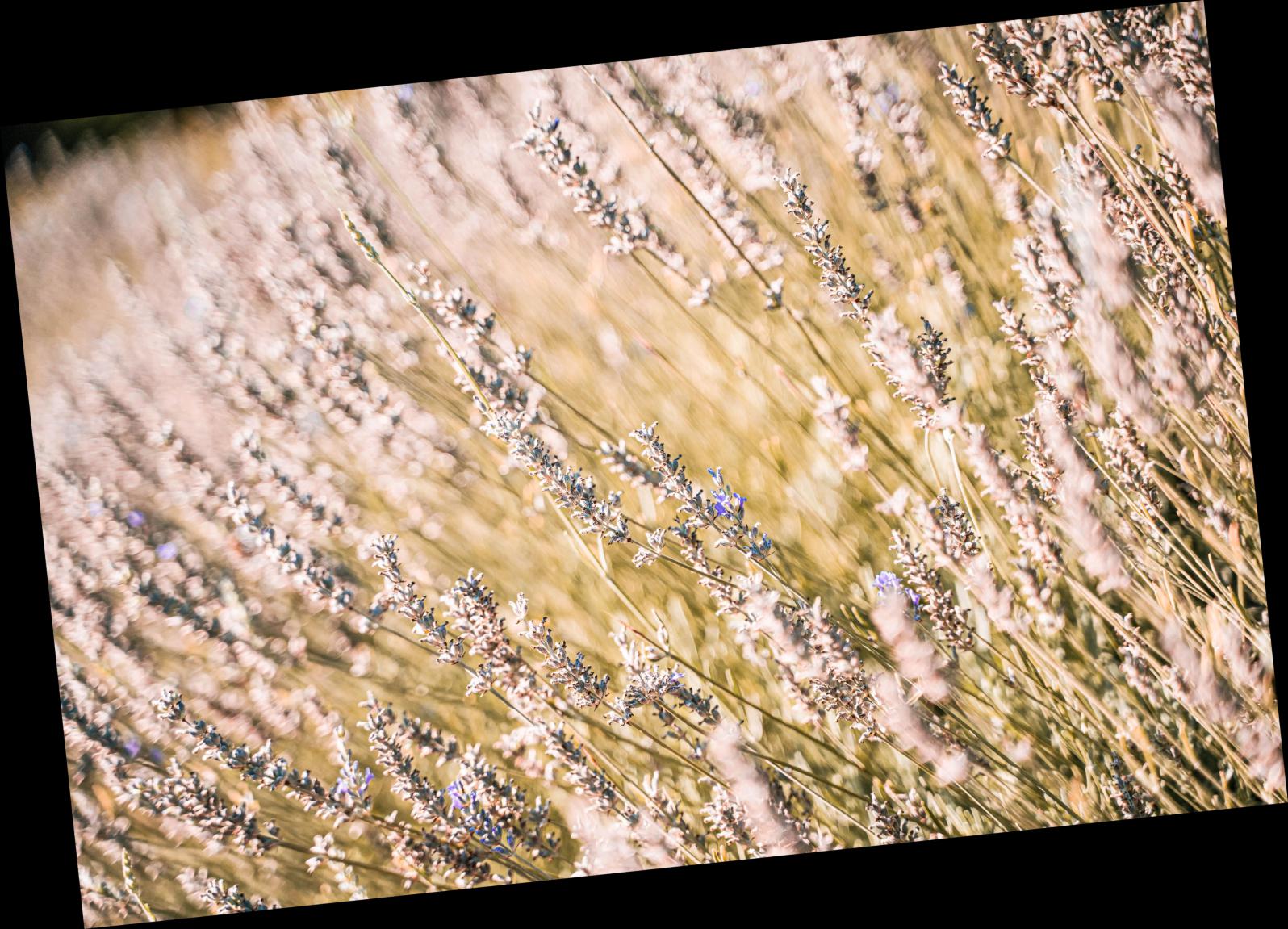
After getting the angles, we can iterate different angles to straighten the image by picking the image that has a good distribution. What I mean by good distribution depends on the image, and we will show a pitfall of this algorithm.
|
|
|
|
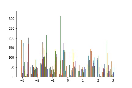
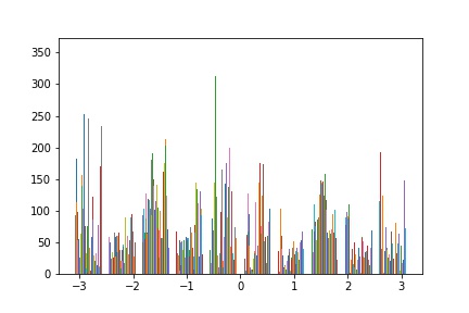
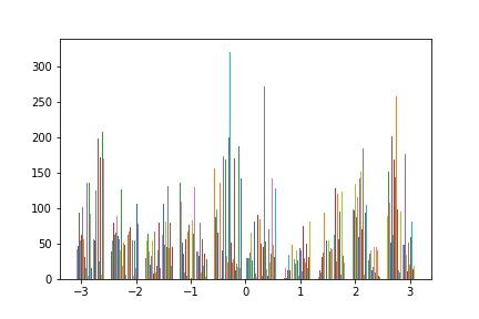
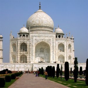
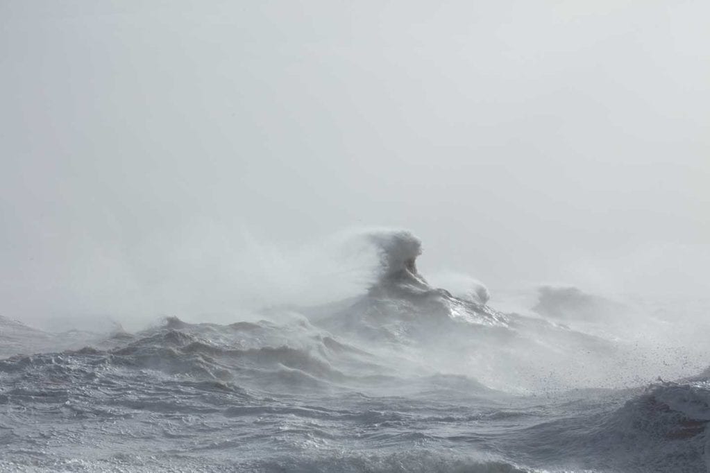
Since the original image is not too different from the straightened version, the histogram between the twos are very close. However, if you look at the value at PI, the straightened image has a higher number of pixel at the PI bucket which is the desired result because it corresponds to the case when the edge is vertical.
|
|
|
|
|
|
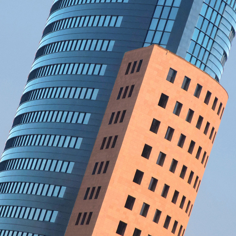
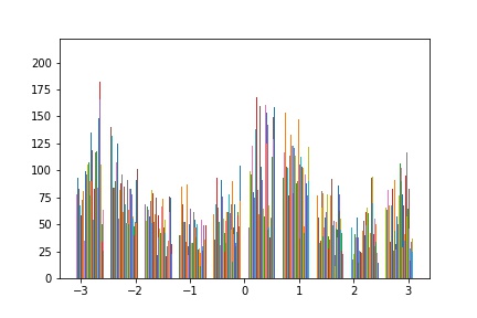
So far so good, we now show a bad example.
|
|
|
In this image, the algorithm fails to straighten the image because the image has a broad distribution.
Now we will extend our frequency knowledge to sharpen an image. The idea behind is that we can add the gaussian-filtered-out content back to the original image to "sharpen" the image.
|
|
|
|
|
|
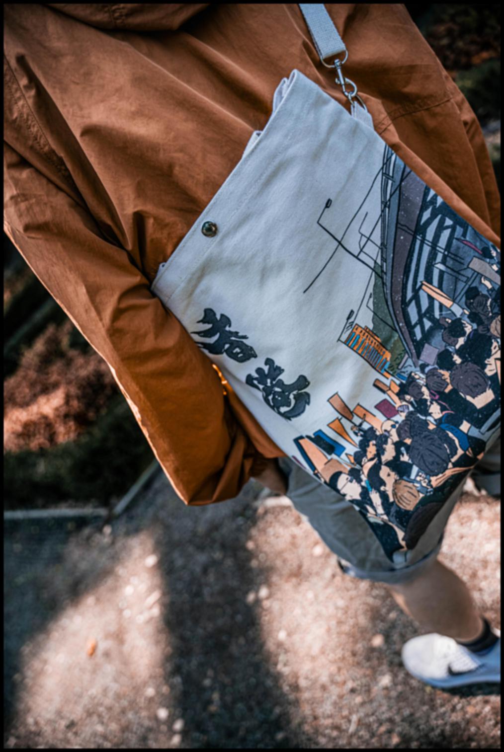
For fun, we want to check if the image is the same if we first blur it then sharpen it again.
|
|
|
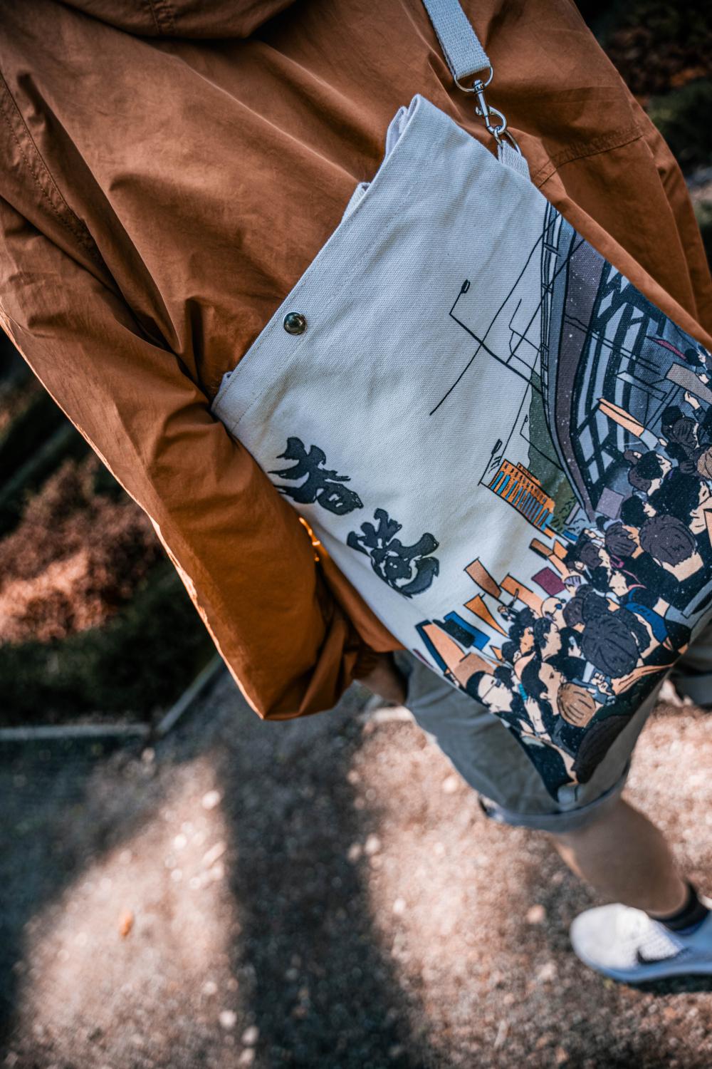
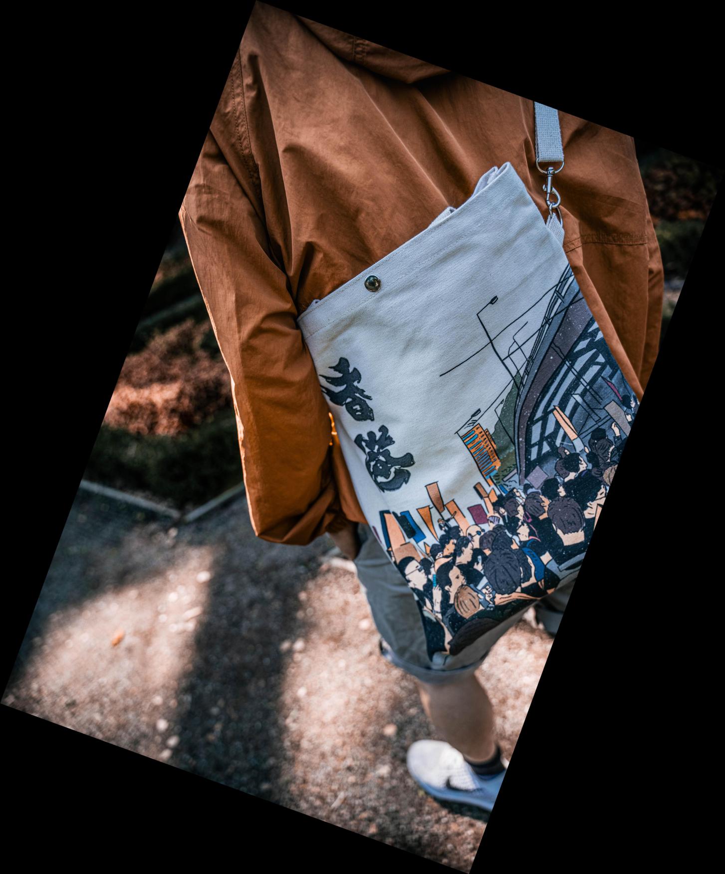
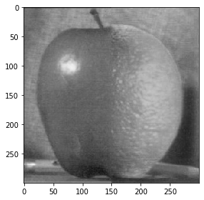
Without doubt, the resharpen image should not look the same because the high frequency image content is lost forever after the image is blurred. We can verify this by looking at the Moire Pattern in the original image (bag) while you can't in the resharpen version.
You might think this frequency stuff is super useful already, but you are wrong, the best is yet to come!
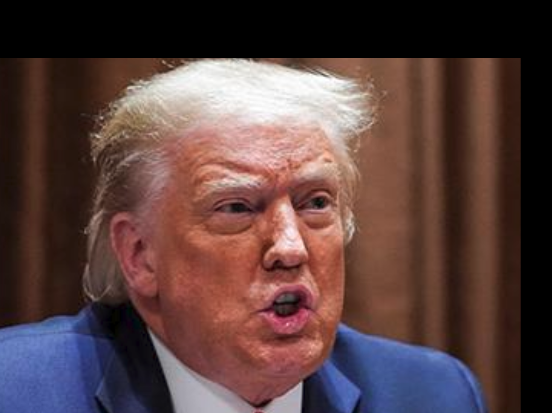
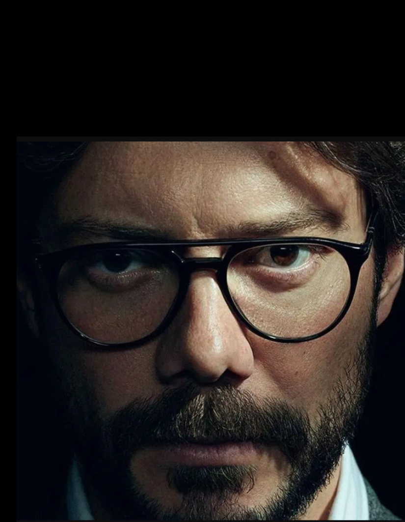
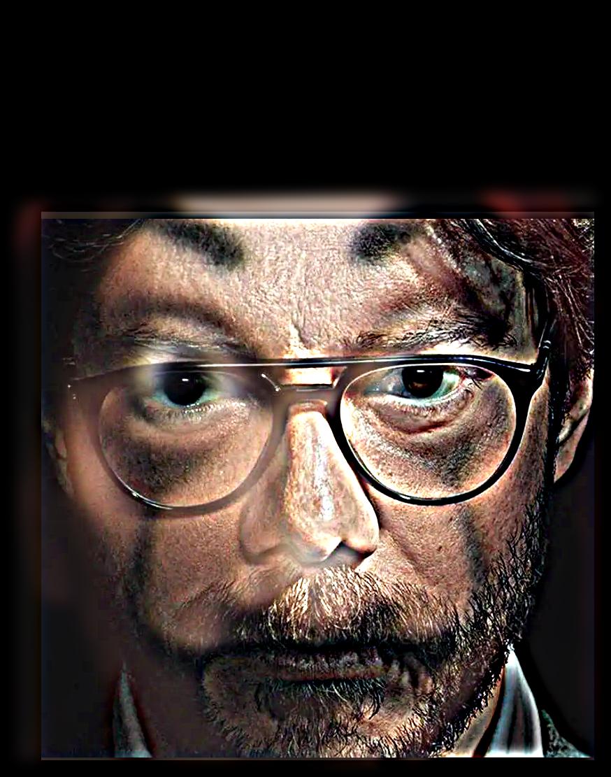
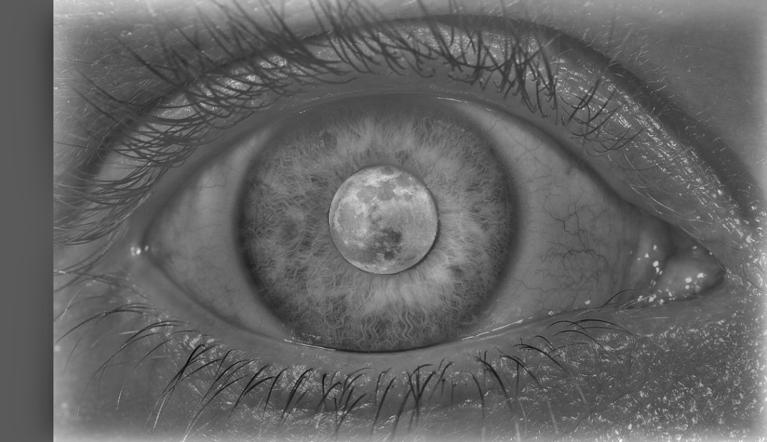
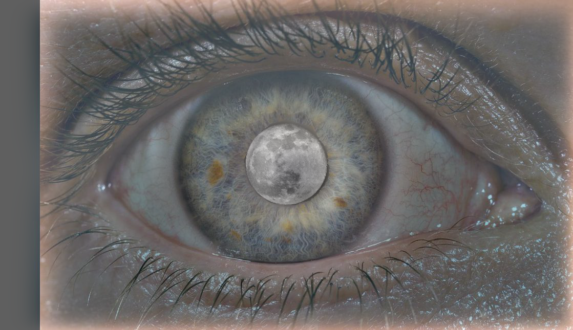
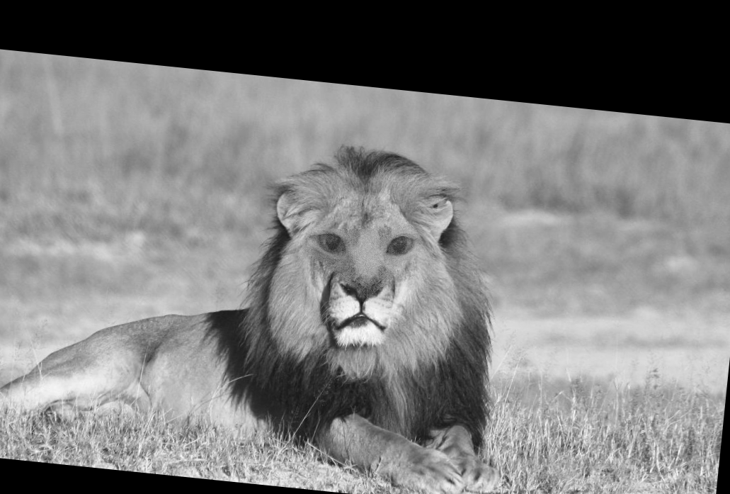
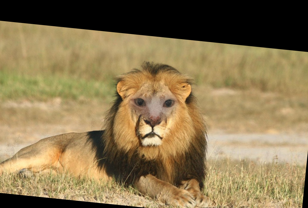
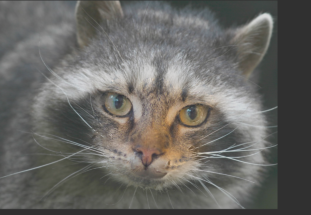
What we are going to do is to overlap two images together such that you could observe one image when you are close while the other when you are far away. This idea is based on the intuition that human usually concentrates on high frequency content when looking at close-up stuff. On the other hand, if we are further away from the image, the high frequency content becomes so small that we can't differentiate the detail. Therefore, if we overlap a low frequency image, the low frequency will become high frequency content from far away, thus the hybrid effect.
|
|
|
|
|
|
|
|
|
|
|
|
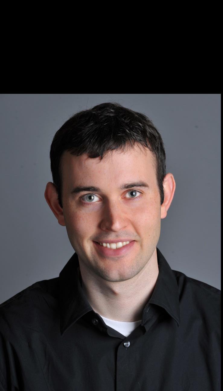
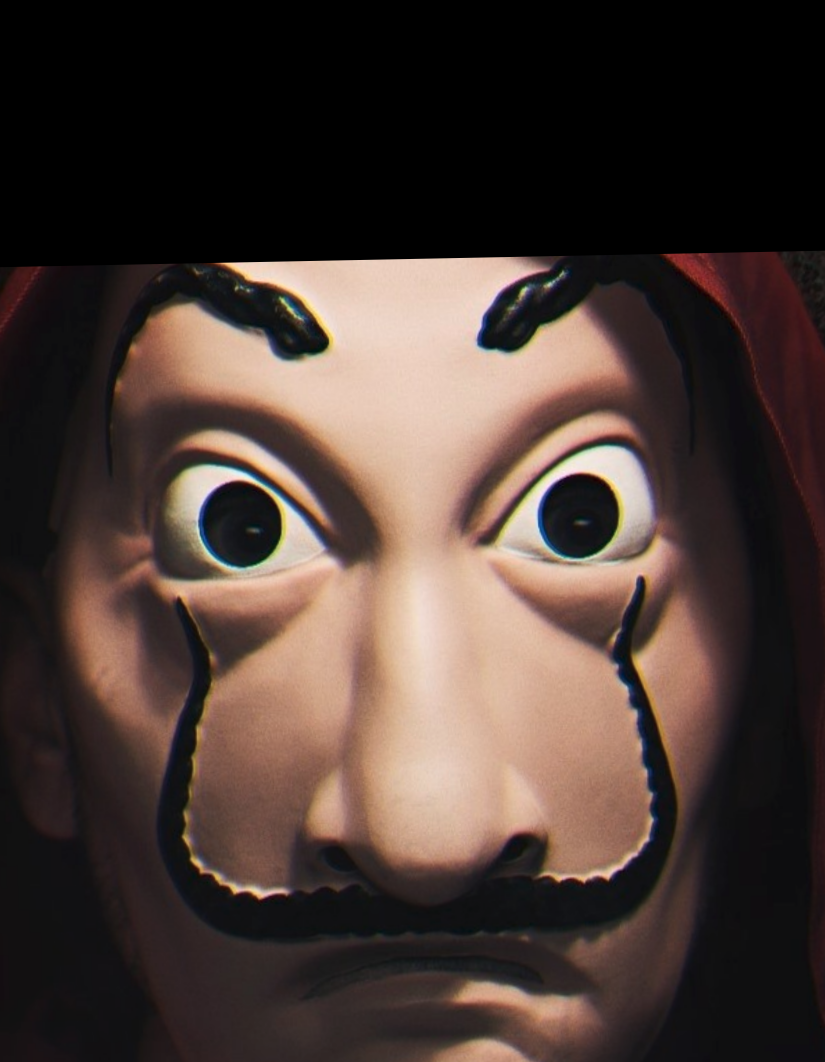
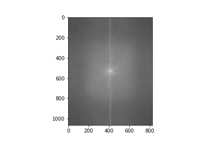
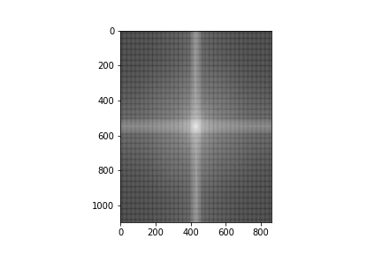
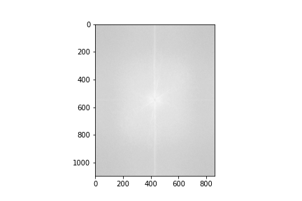
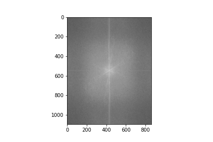
In order to further understand this algorithm, we want to analyze the image in fourier domain. Taking the mask and professor as an example.

|
|
|
|
|
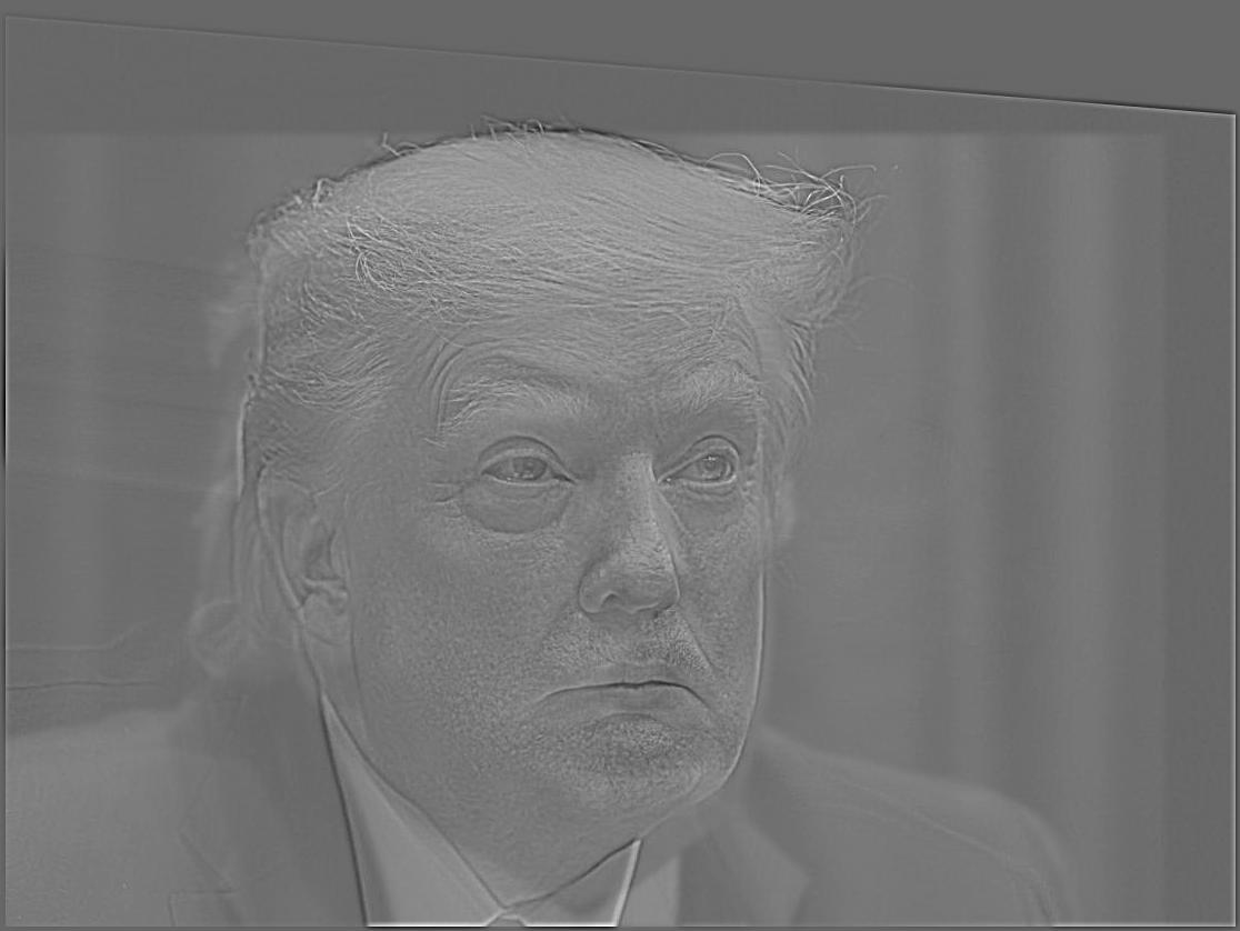
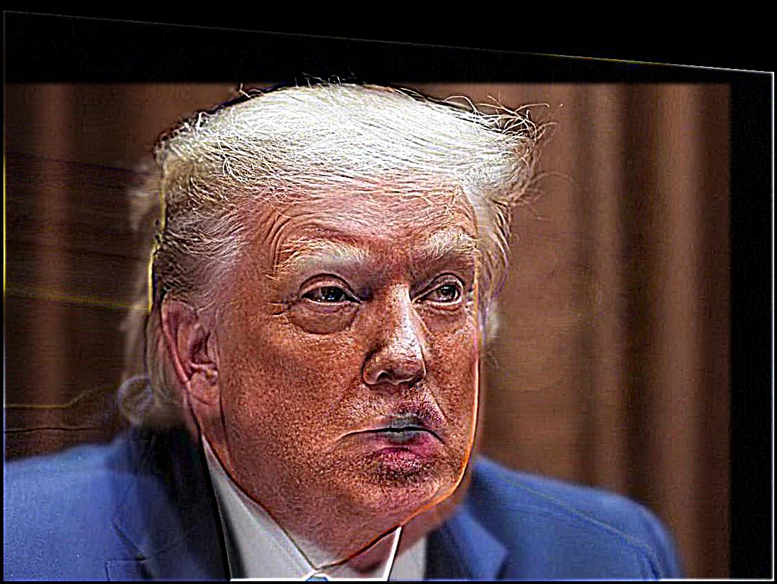
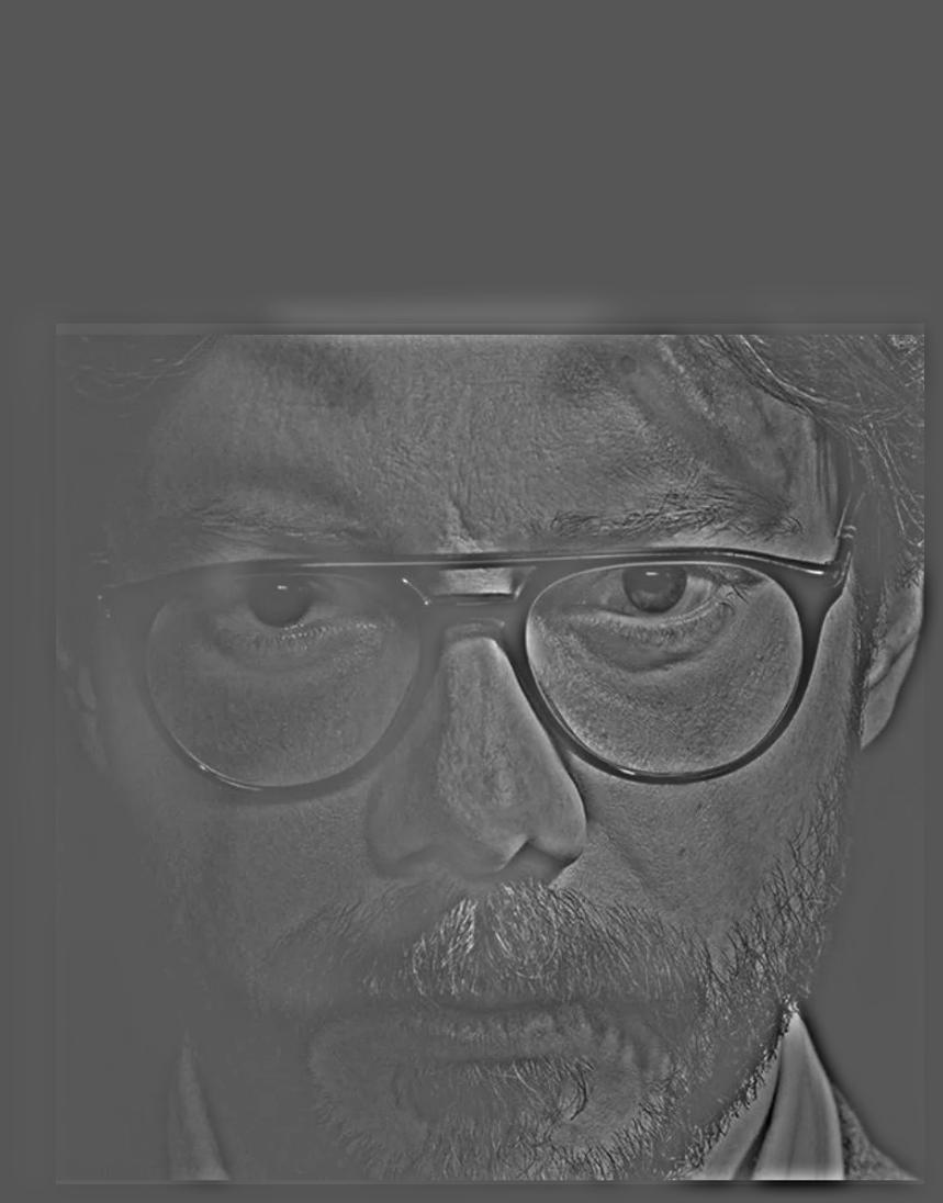
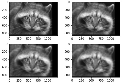
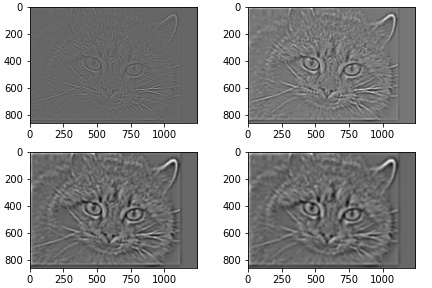
Analyzing the image in fourier domain is not too intuitive, is there any other analysis we can perform instead. We are in luck, Laplacian and Gaussian Stacks are here to help. The idea of stack and pyramid is similar except we don't downsample the image in a lower level. Gaussian stack is simply a stack of incrementally blurred images. More specifically, the first level is the original image, the second level is a blurred version of the image convolved by a filter at w_cutoff, the third level is the second level image convolved by the same filter, and so forth. Now, we have a stack of incrementally blurred images, we can do a subtraction in between every two levels of images to extract the filtered content (from high to low frequency).
|
|
|
|
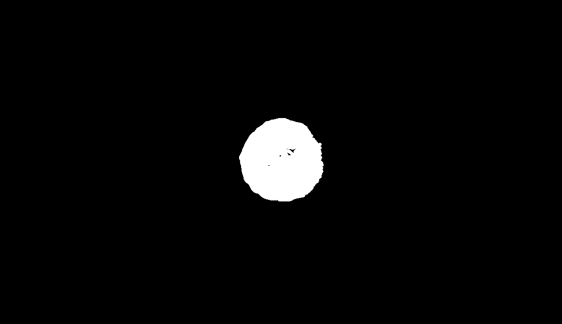
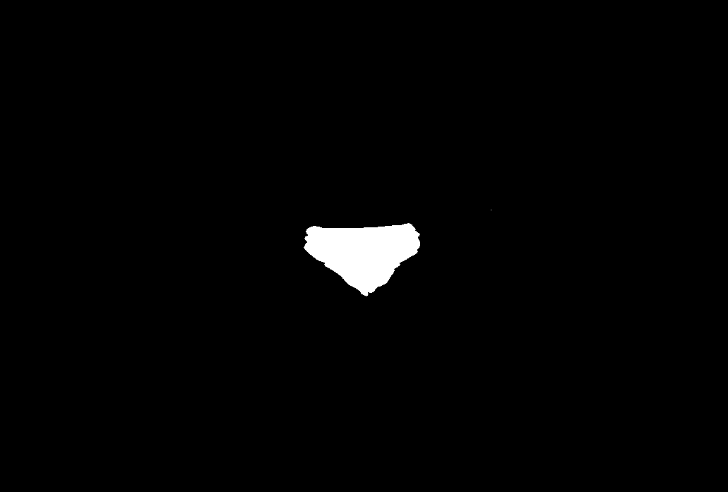
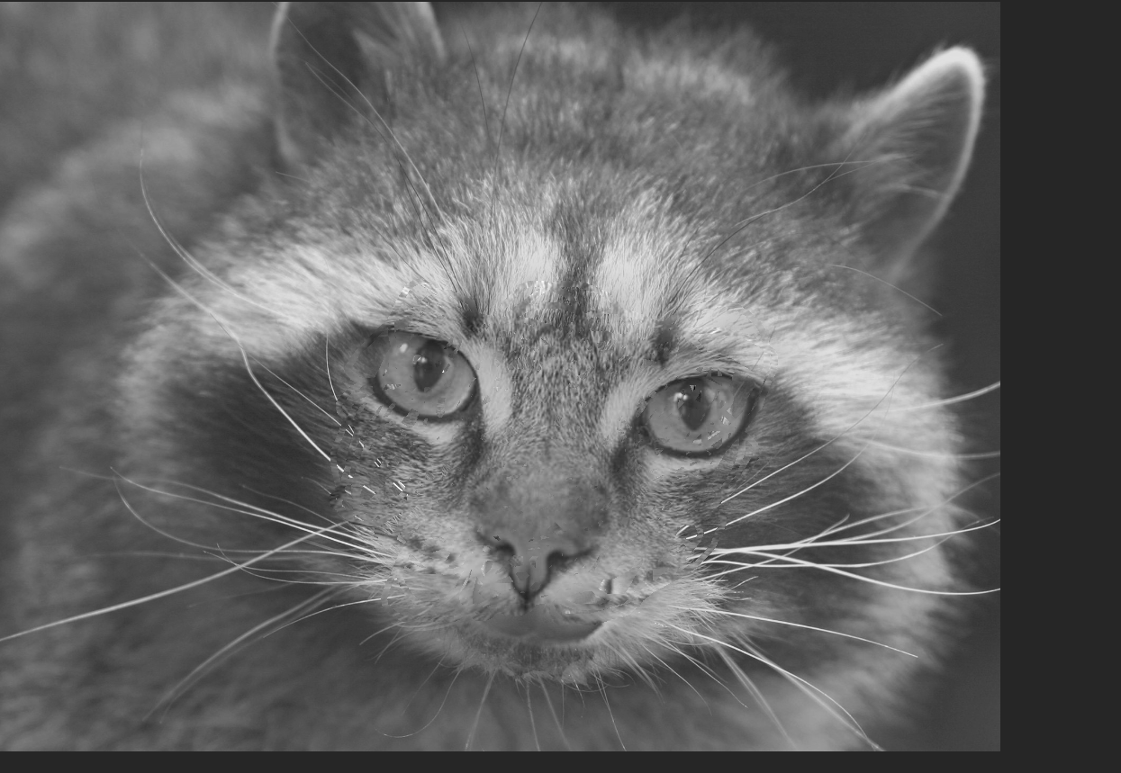
If you had enough frequency fun, you never had enough frequency fun. We are going to blend two images together such that we are not going to see the hard edges in the overlapped region. The idea is really simple: we are going to slice the image into different frequency bands such that the frequency of the most prominent feature is around the two times the frequency of the least prominent feature in that band of image. In this way, we can perform blending with higher granularity. The most important part of this part is to create a binary mask to crop out objects you want to blend. We can then use gaussian filter to smooth out the masks such that the higher frequency component will have less feathering while the lower frequency component will have more.
|
|

|
|
|
|
|
|
|
|
|
|
|
|
This homework is insanely enjoyable to implement and play around with. The raccon and cat blending image is insane. After this homework, I understand more about the photoshop features and how easy it is to create fake images.