The goal of this project was to implement image blurring using a Gaussian Kernel, image straightening by counting horizontal/vertical edges, image sharpening, hybrid images, gaussian/laplacian stacks, and multiresolution blending.
Part 1: Fun With Filters
Part 1.1: Finite Difference Operator
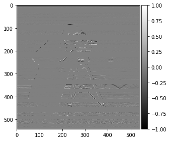
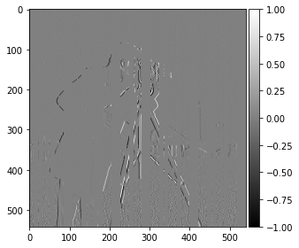
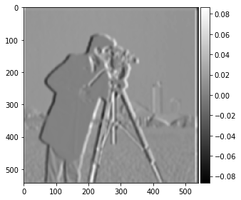
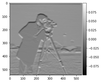
The partial derivative in x and y were taken of the cameraman image by convolving the image with the finite difference operators.
partial derivative in xpartial derivative in y
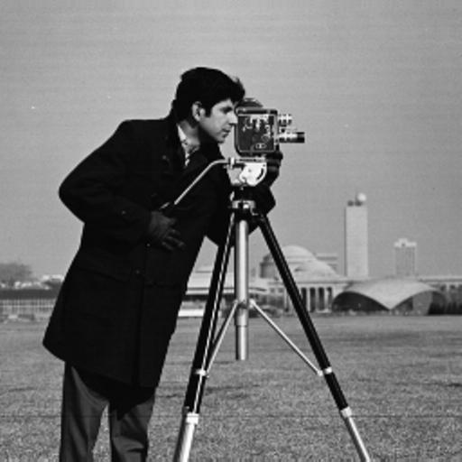
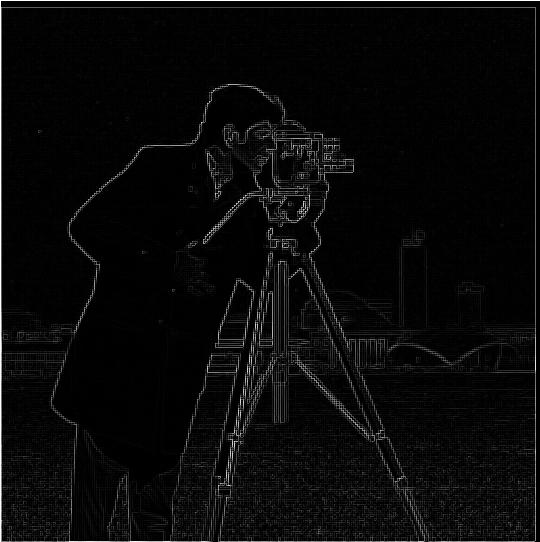
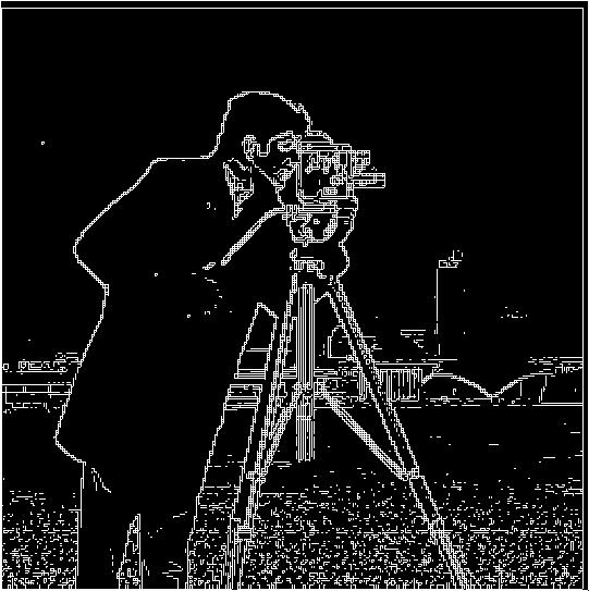
The next step was to compute the gradient magnitude image, which is done by taking the square root of the sum of the squares of the derivatives in x and y. Then, the gradient magnitude image was converted into an edge image by binarizing the pixel values, giving values less than a threshold of .14 to 0, and 1 otherwise.
original cameraman imagegradient magnitude imageedge image
Part 1.2: Derivative of Gaussian (DoG) Filter
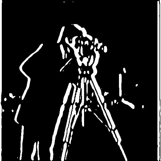
It is apparent that there is a lot of noise in the edge image produced. This is fixed by applying a gaussian blur by convolving a gaussian kernel with the edge image. The convolution from the previous part can be convolved with the gaussian kernel to create a single convolution that produces a better edge image. The white dots/noise created from the grass in part 1.1 is now removed.
edge image with gaussian blurpartial derivative in xpartial derivative in y
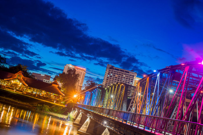
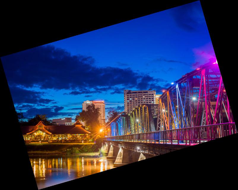
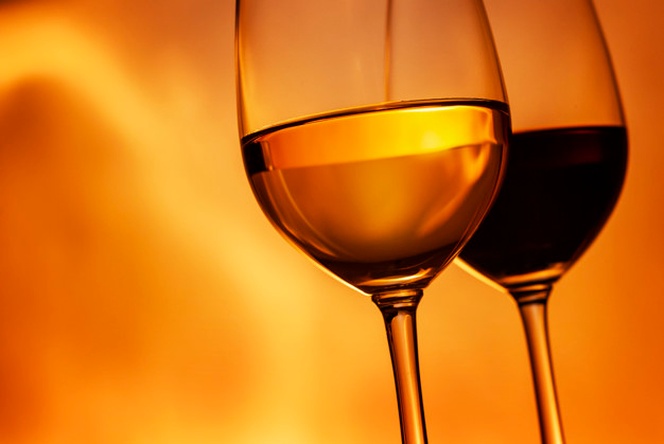
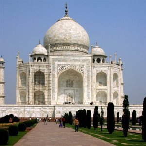
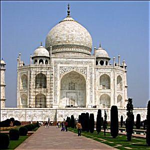
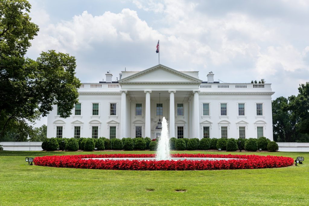
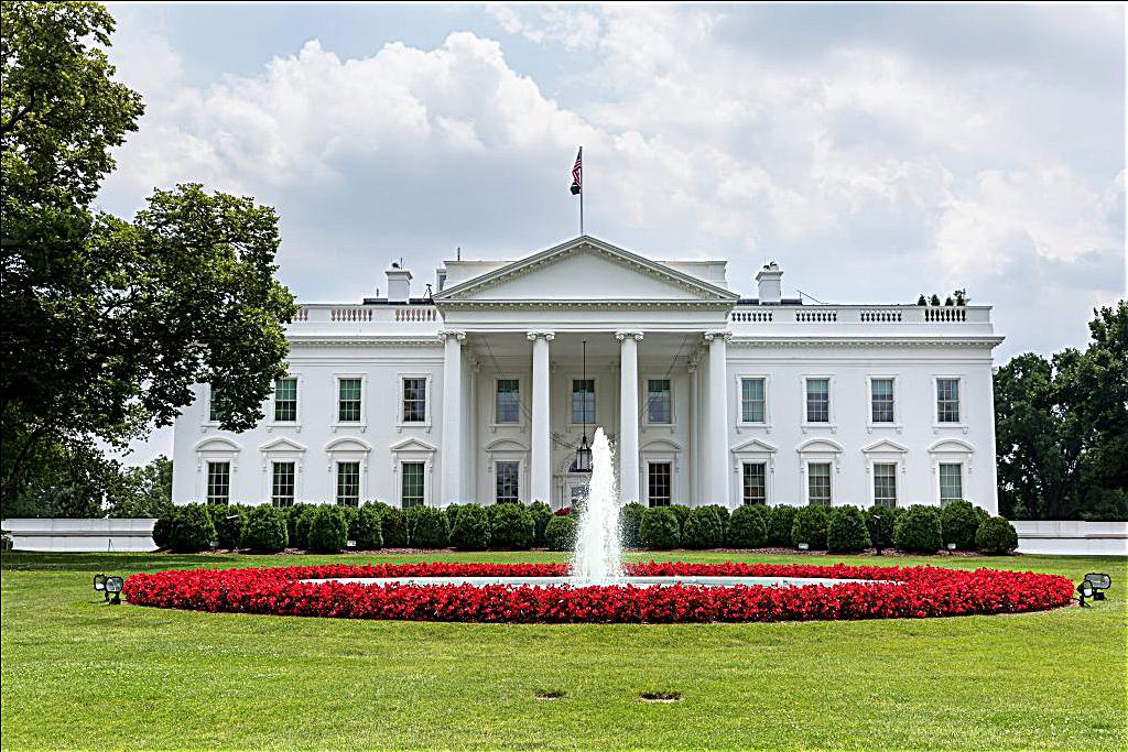
Part 1.3: Image Straightening
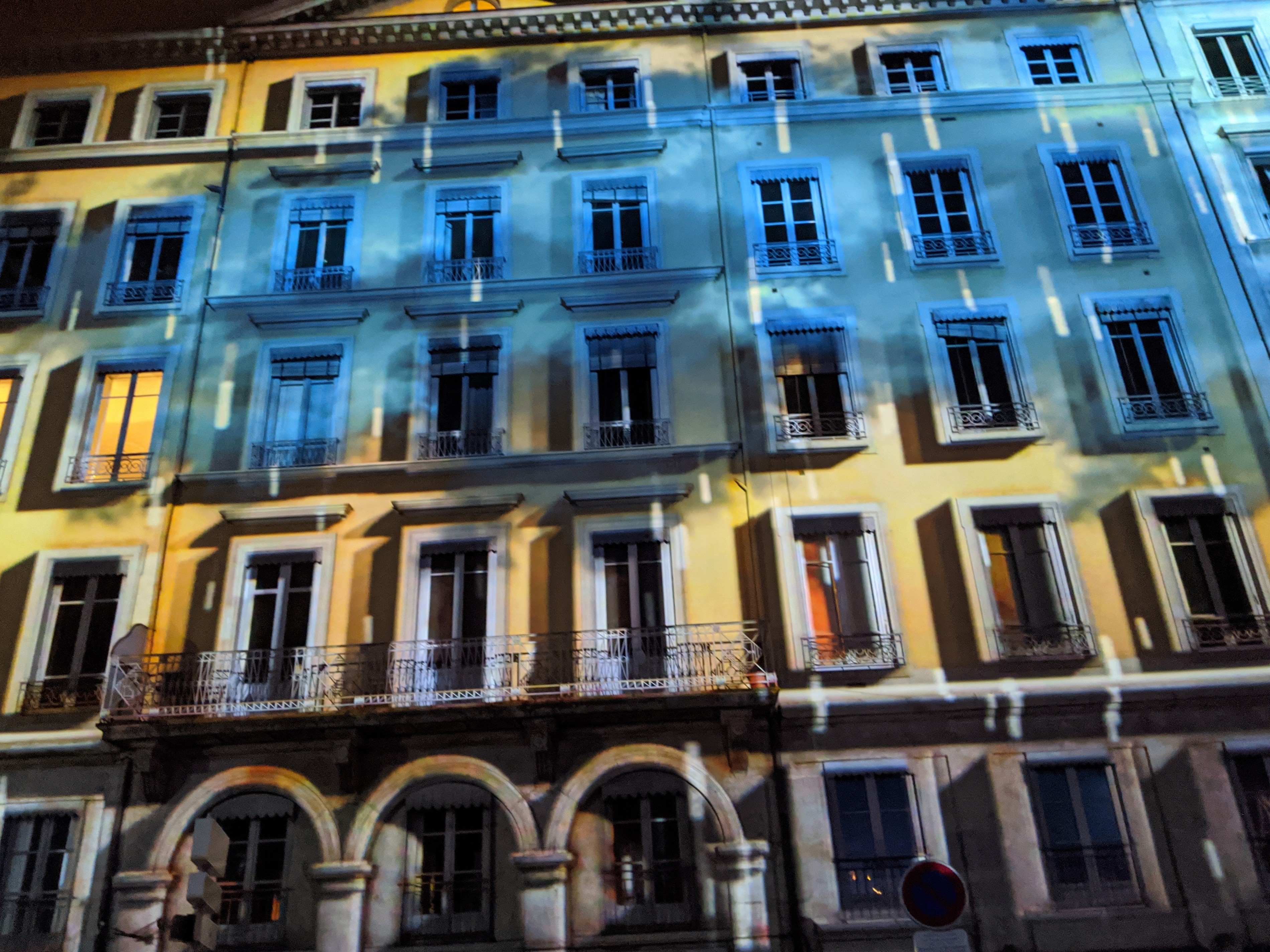
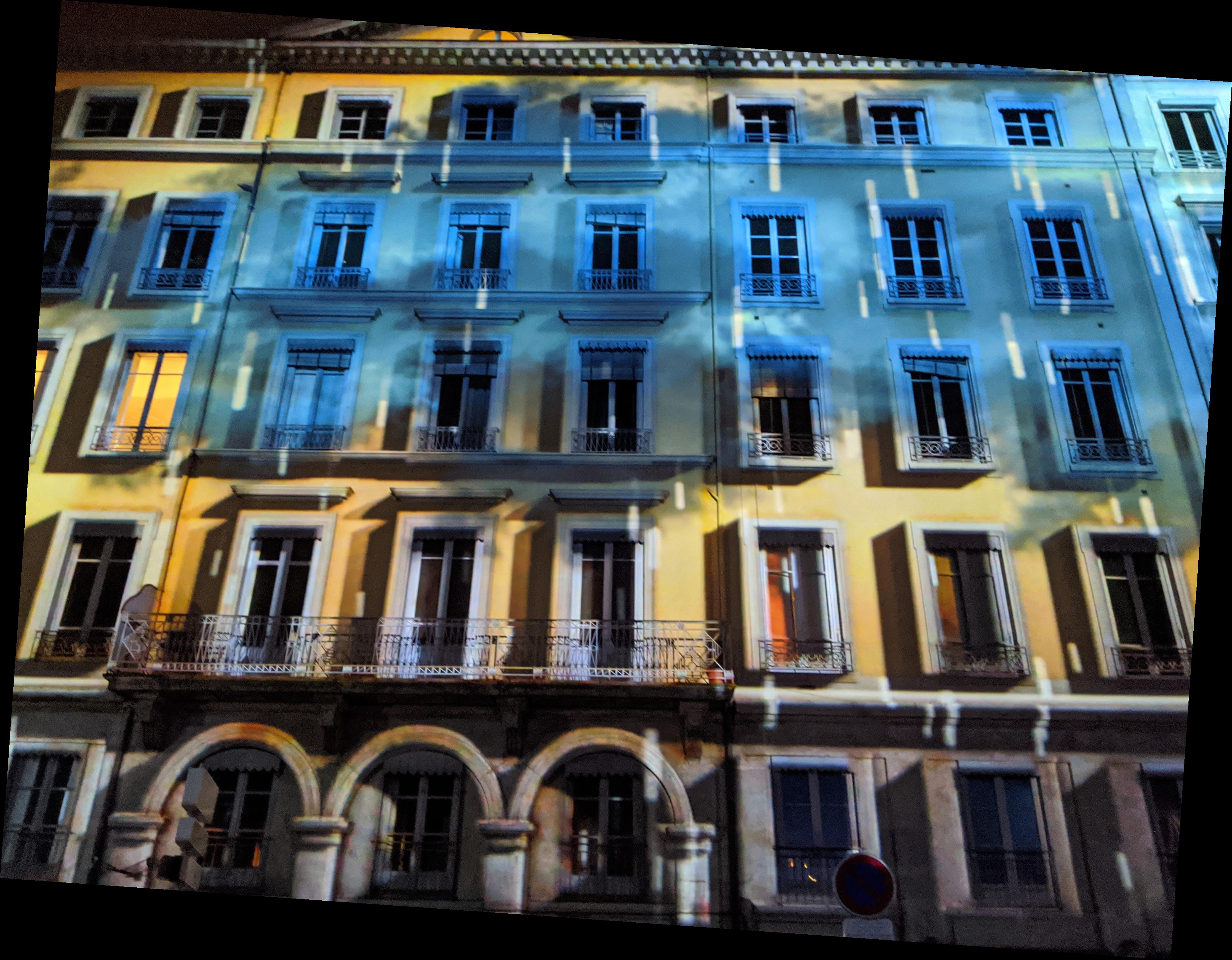
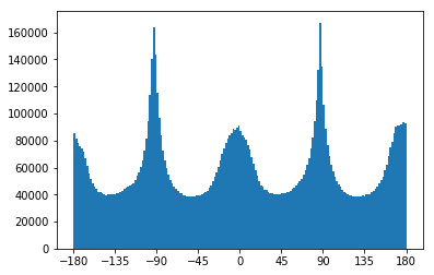
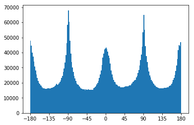
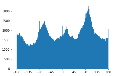
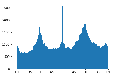
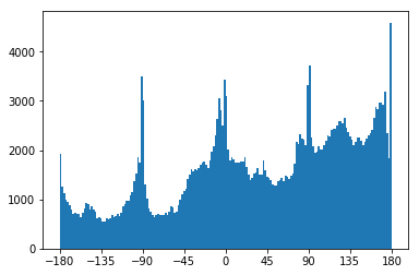
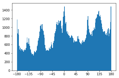
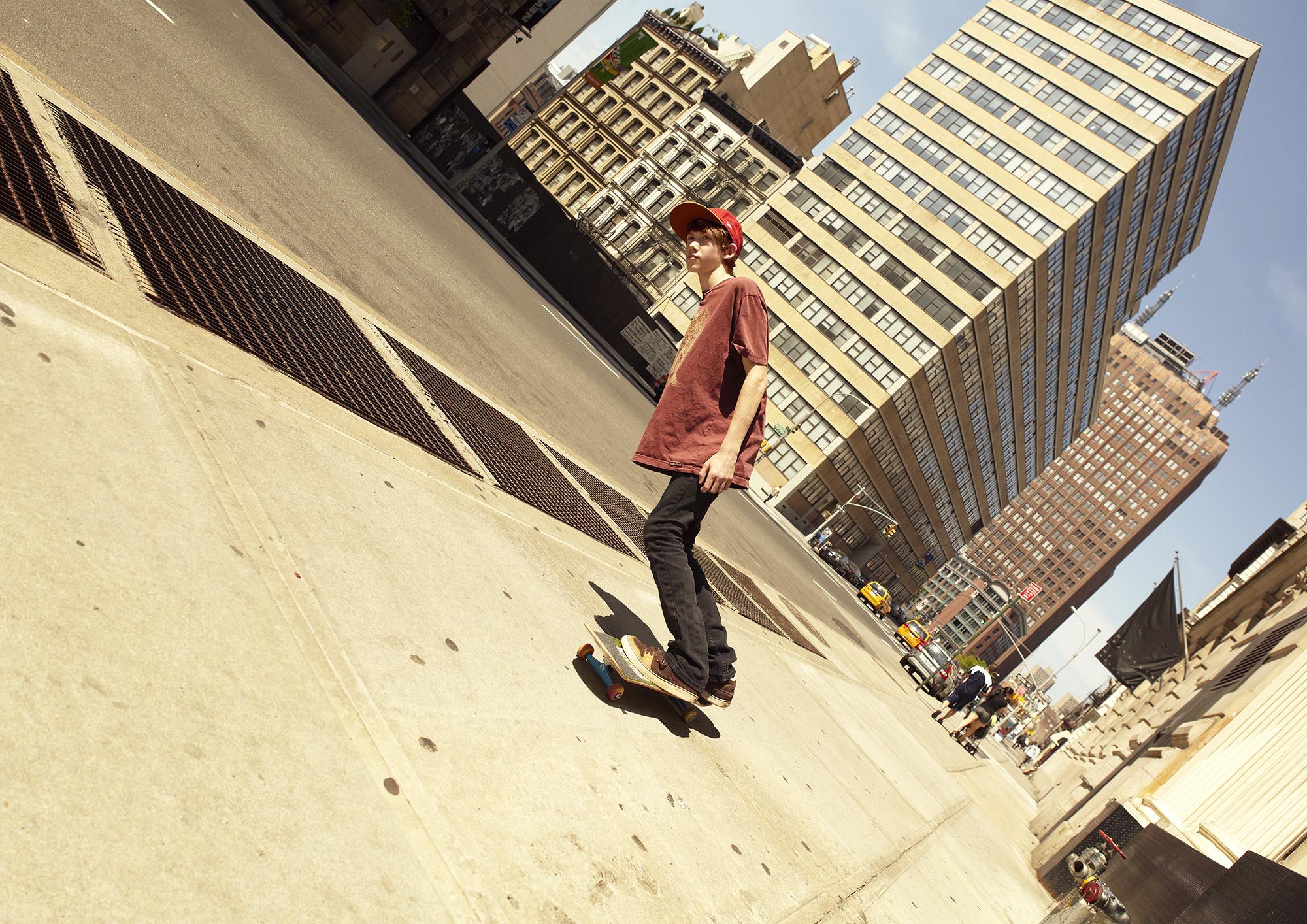
In order to automate the image straightening process, I first rotate the image by a certain degree in a predetermined range [-20, 20). Since a rotation creates unneeded empty space in the image, I cropped out the outer fifths of the image and only used the center when calculating the gradient angles using the formula arctan2(dy, dx). dy and dx were the partial derivatives of the image, calculated similarly to part 1.1. I then count the number of gradient angles that are within +/- 2 degrees from 90 and 180 degrees for each rotation, and take the maximum count in order to maximize the number of horizontal and vertical edges.
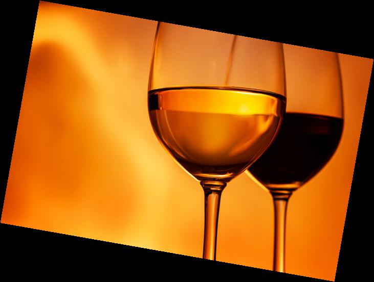
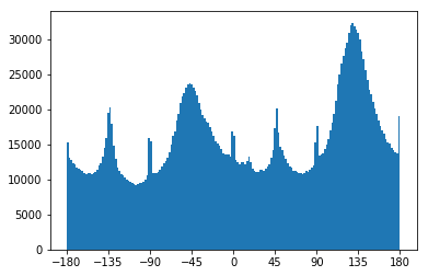
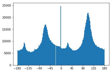
original imageimage rotated by -4 degreeshistogram of gradient angles of original imagehistogram of gradient angles of rotated image
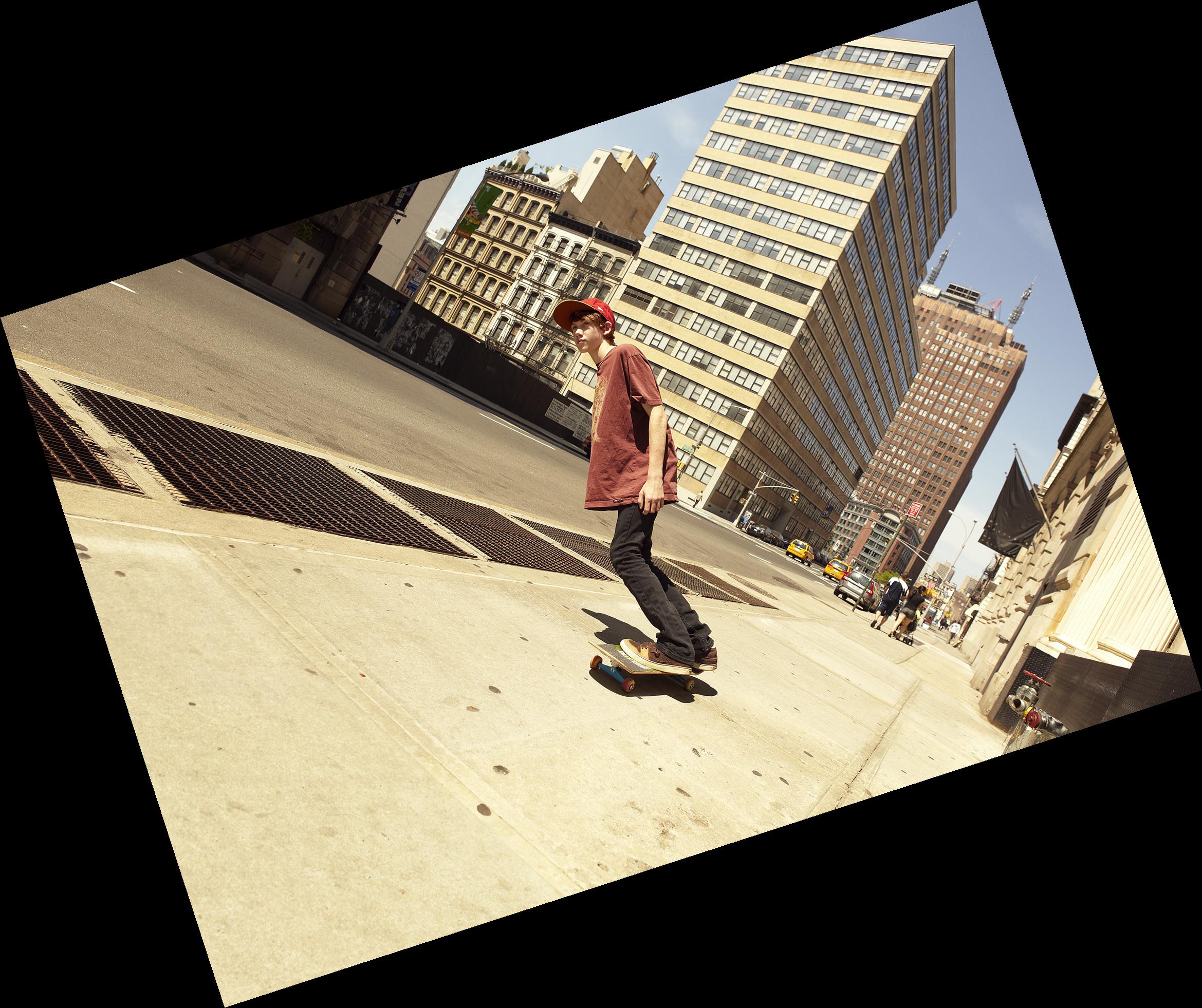
original imageimage rotated by -18 degreeshistogram of gradient angles of original imagehistogram of gradient angles of rotated image
original imageimage rotated by -18 degreeshistogram of gradient angles of original imagehistogram of gradient angles of rotated image
This picture probably failed because there were multiple perspectives of straight, from the ground to the kid to the buildings behind. It also likely that the rotation range is out of the one i provided.
original imageimage rotated by -18 degreeshistogram of gradient angles of original imagehistogram of gradient angles of rotated image
Part 2.1: Image "Sharpening"
In order to "sharpen" an image, we can take the high frequencies of the original image, computed by subtracting its gaussian blur from itself, and it to itself. Enhancing the high frequencies gives the illusion of a sharper image. All of these steps can be combined into a single convolution operation, with the convolution matrix being (1+alpha) * unit_impulse - alpha * gaussian_kernel. I chose alpha to be 1.
original imagesharpened image with guassian kernel of size 10 sigma 2
original imagesharpened image with guassian kernel of size 10 sigma 2
original imageblurred imagesharpened blurred image with guassian kernel of size 10 sigma 2
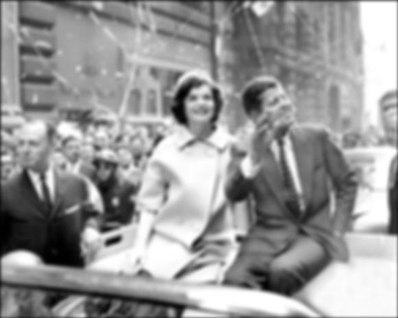
After the JFK image was blurred, attempting to sharpen the image did not produce a result that was close to the original. This is likely because the original blurring removed many of the high frequencies, which would reduce the effectiveness of the image "sharpening" process.
Part 2.2: Hybrid Images
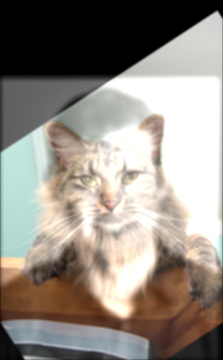
To combine two images together, I take the low frequencies of one image and combine it with only the high frequencies of the other. This results in an image that more closely resembles the high frequency image when looked at closely, and more closely resembles the other when seen from a distance. The low frequencies are obtained through a gaussian blur, and the high frequency by subtracting the low frequencies from the original image.
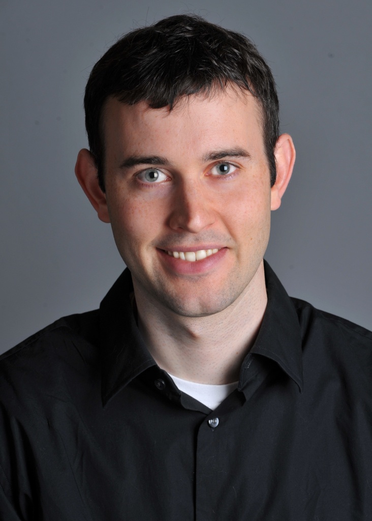
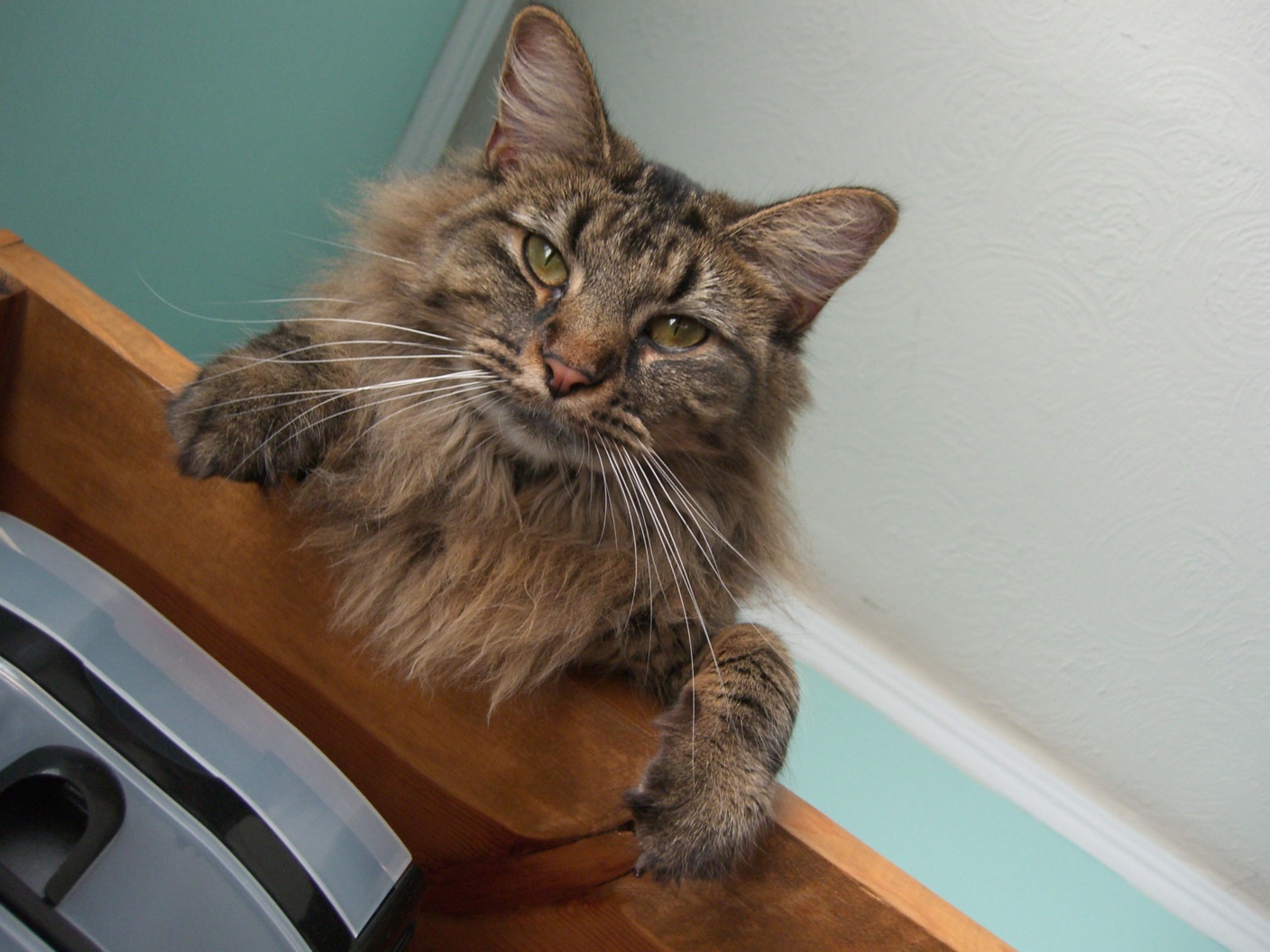
Derk and a cat
input imageinput imagehybrid image
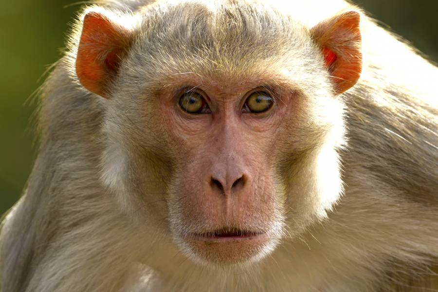
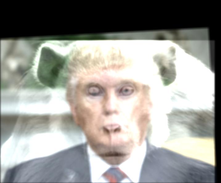
Trump and a monkey
input imageinput imagehybrid image
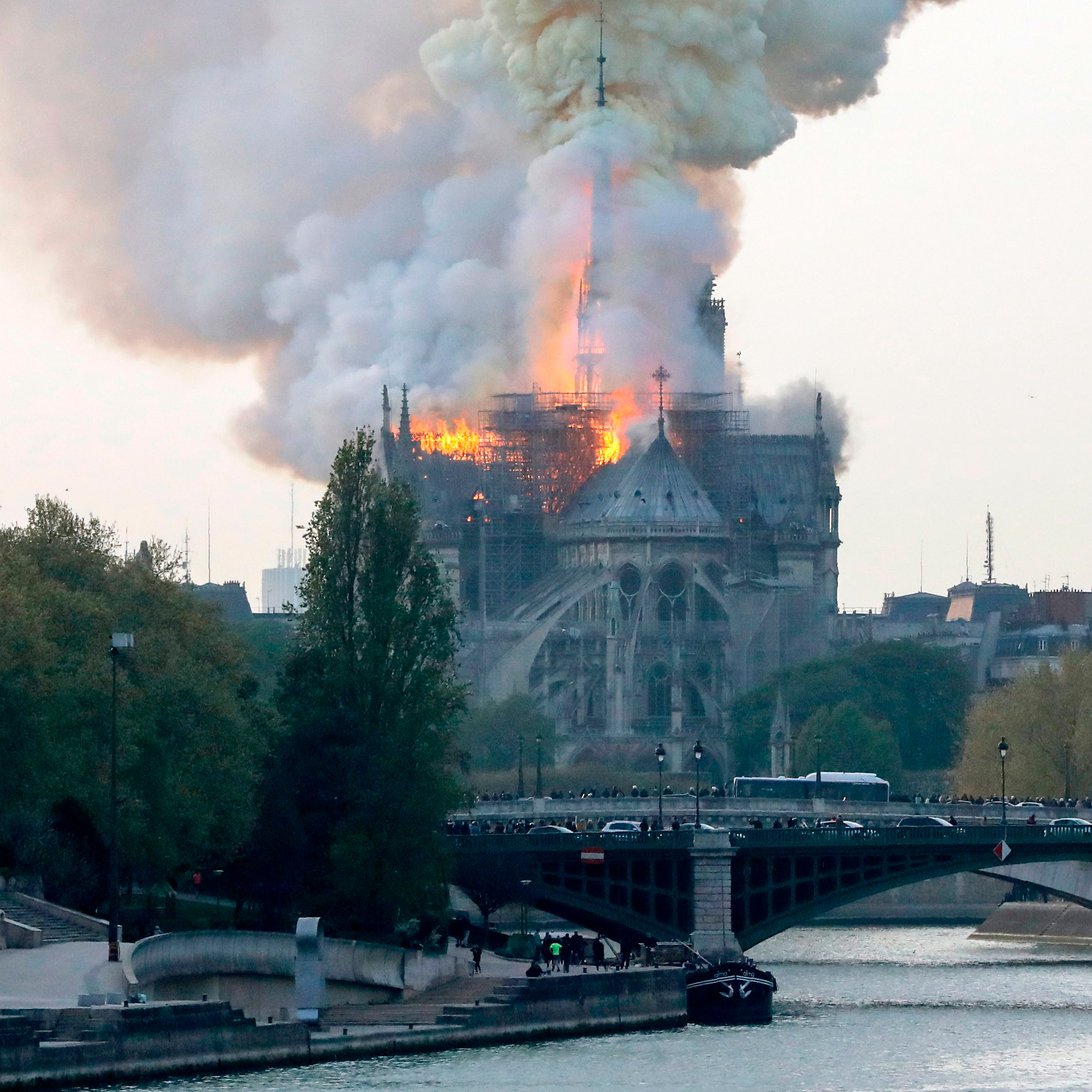
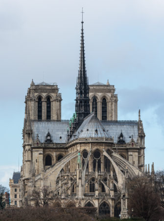
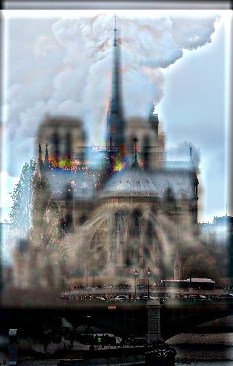
A burning and non burning Notre Dame
input imageinput imagehybrid image
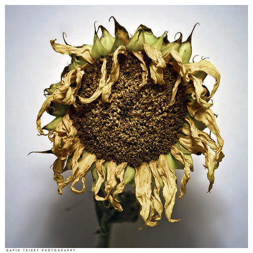
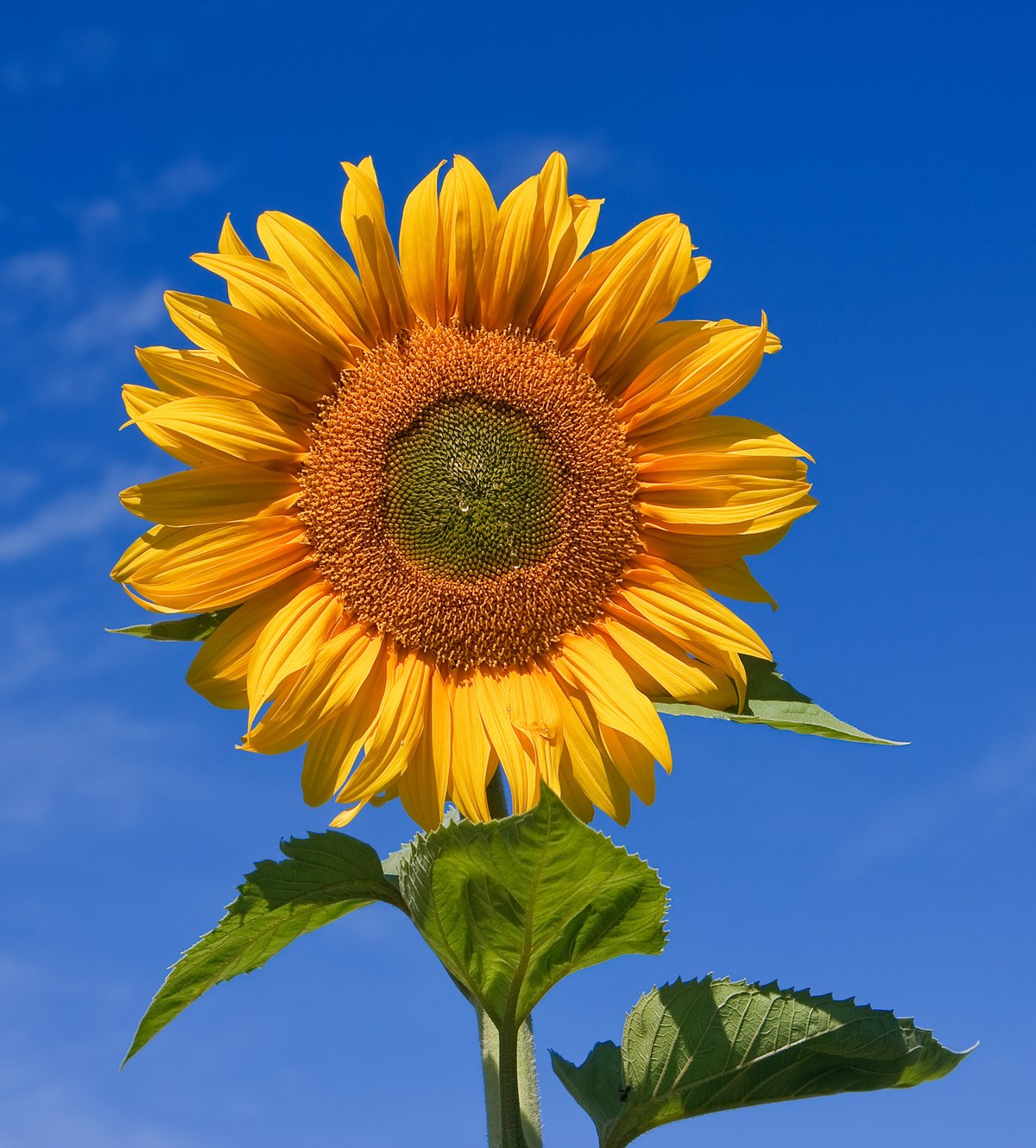
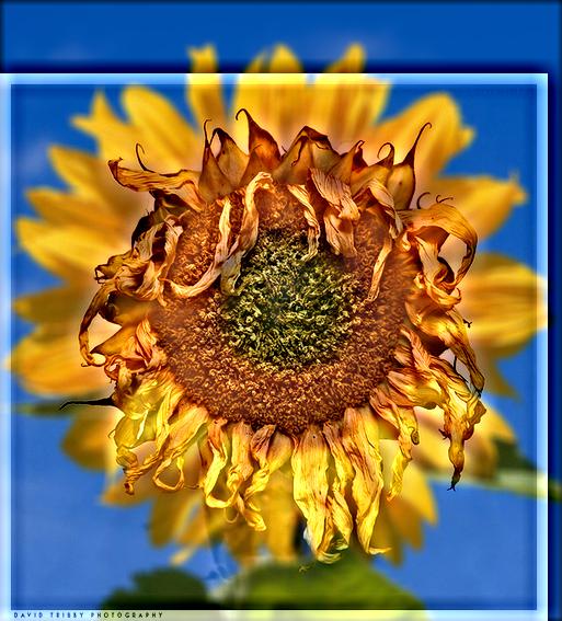
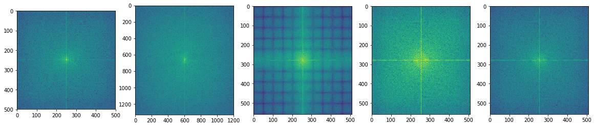
A dead and healthy sunflower
input imageinput imagehybrid imageFFT of, from left to right: input 1, input2, filtered 1, filtered 2, hybrid
Bells and Whistles
After implementing both grayscale and color hybrid images, I discovered that the quality depended on the input pictures, but it was generally beneficial for the lower frequency to be in color and the high frequency to be in grayscale.
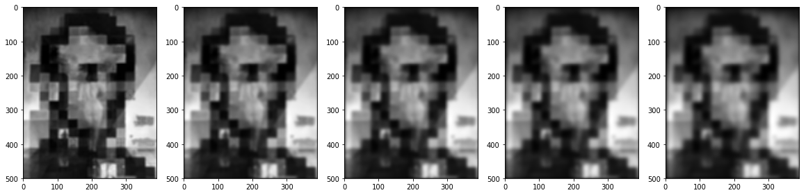
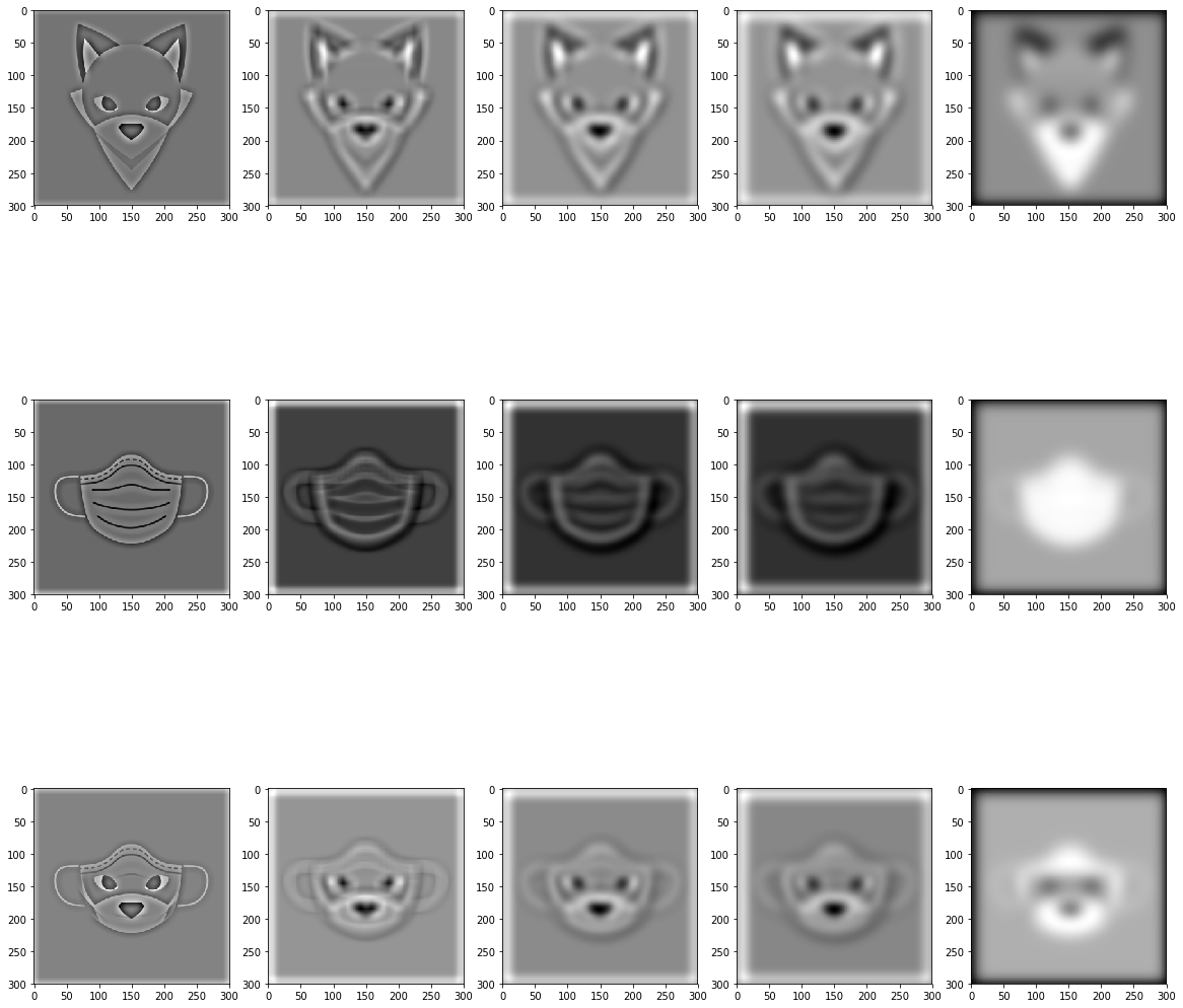
Part 2.3: Gaussian and Laplacian Stacks
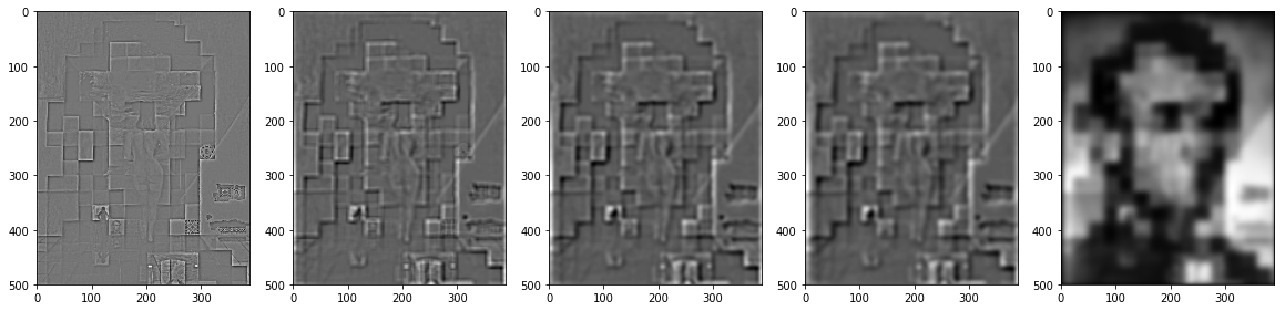
I did not subsample the images on each level because these are Guassian and Laplacian stacks, not pyramids. The process is fairly simple, reusing the gaussian kernel methods from previous parts for the Guassian stack. The Laplacian stack is obtained at each level by subtracting the newly blurred image from the blurred image from the previous level.
Salvador Dali painting of Lincoln and Gala
gaussian stacklaplacian stack
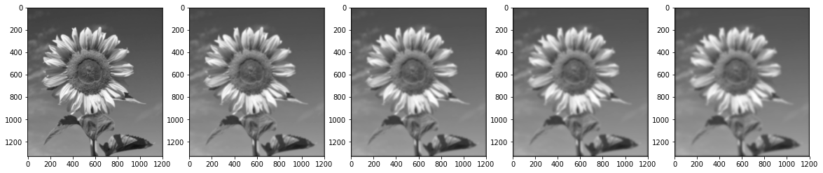
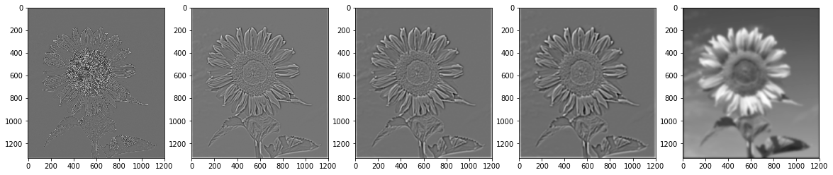
Suflower (from part 2)
gaussian stacklaplacian stack
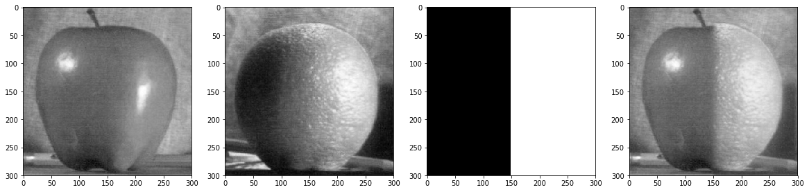
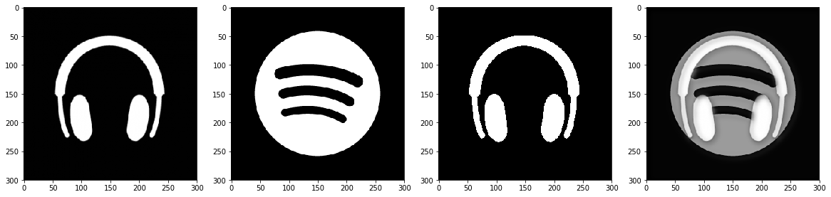
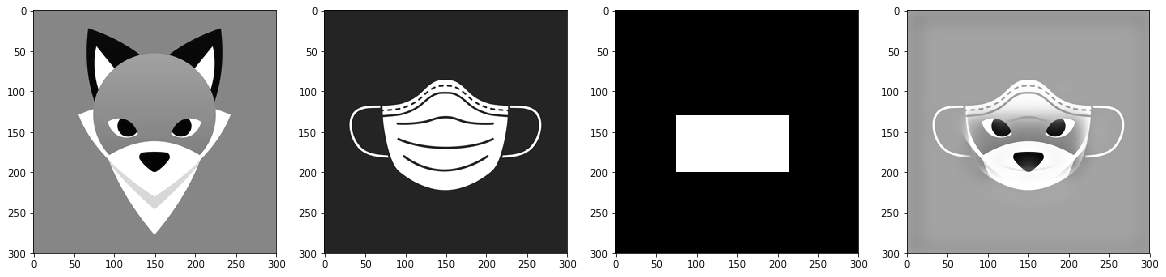
Part 2.4: Multiresolution Blending (a.k.a. the oraple!)
To blend two images together, an image spline is used to smoothly blend the edges(multiresolution blending). A mask is used to outline the edges for blending. To obtain the blended image, we use the gaussian and laplacian stacks of each input image, using the formula LS_i = R[i]*LA[i] + (1-R[i])*LB[i] to calculate the image at each level. Finally, all the levels are summed together.