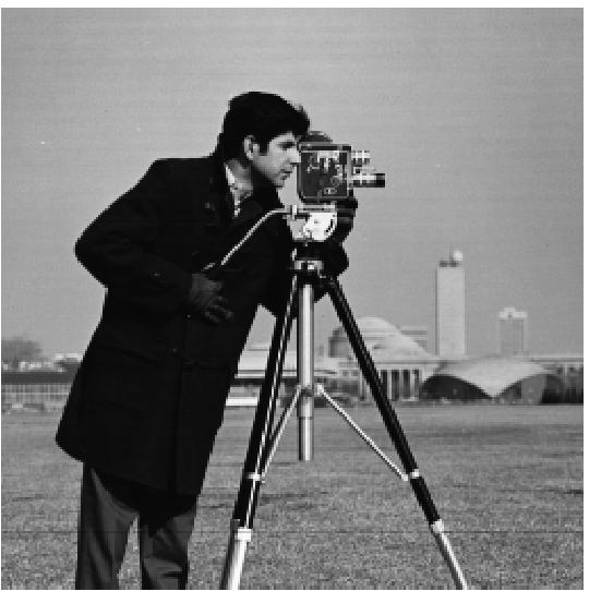
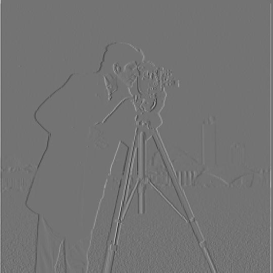
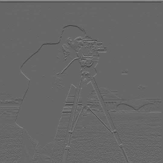
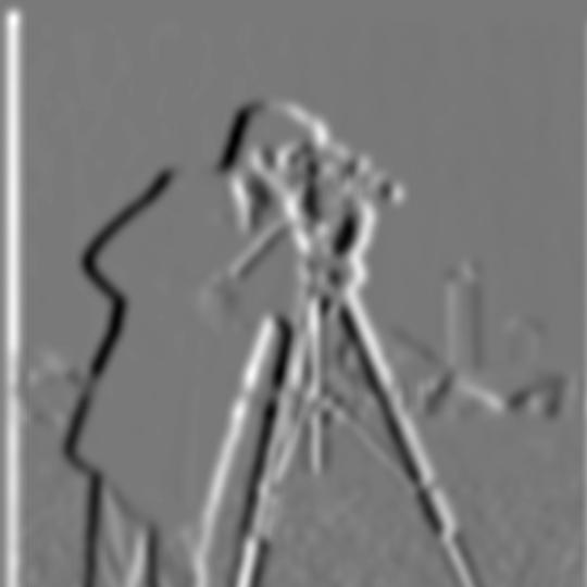
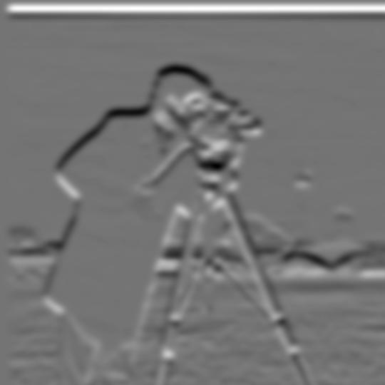
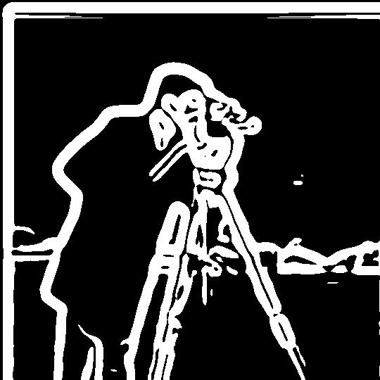
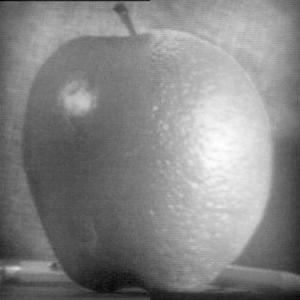
In this part of the project, we will be taking derivatives of the famous camera man image. We can apply derivative filters (of the form [1,-1]) both in the x direction and the y direction. In either case, we will see "outlines" of where color changes rapidly. This is the basis for edge detection.
|
|
|
|
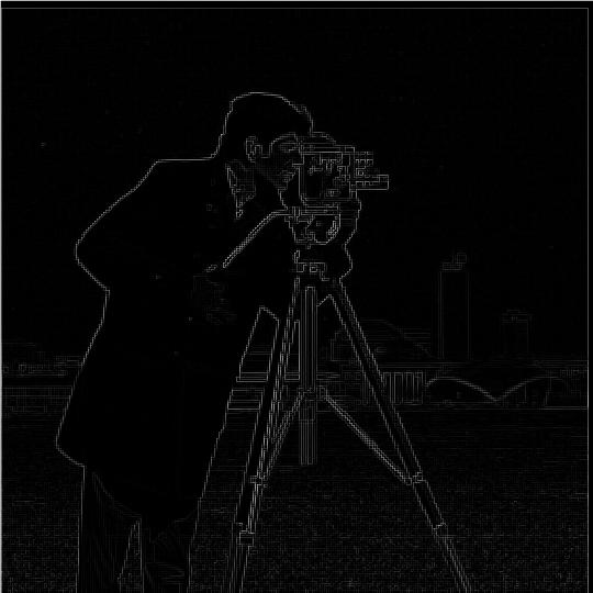
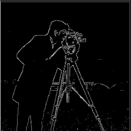
After we compute the derivates of the x and y axes, we can use them to compute the gradient magnitude. To do so, we square the x and y derivatives, add them together, and square root the result. What we get is an outline of positions where the derivates were most active. After we have the gradient magnitude, we can binarize it by assigning a 0 or 1 mapping to pixels below or above a certain threshold.
|
|
|
|
Although we can see the edges of the camera man, they could be more prominent. What we will do is now compute a Gaussian filter. Then, we will convolute the Gaussian filter with the finite difference operators from 1.1 to obtain derivative filters that can capture more gradual change.

|

|
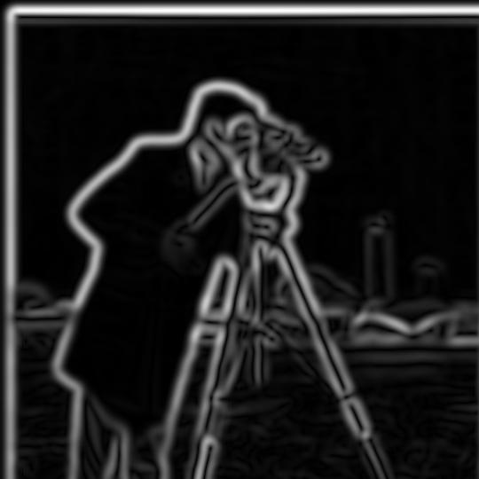
These Derivative of Gaussian (DoG) filters will allow us to emphasize the edges in our image a bit better than before with the finite difference operators.
|
|
|
|
We compute the gradient magnitude and binarized gradient in the same manner as before.
|
|
|
|
When using a Gaussian filter instead of finite difference filters, we see that out camera man's gradient magnitude is significantly "thicker". This is due to the fact that we smooth the image with our Gaussian filter. By smoothing the image, we in turn smooth the edges which makes them larger! In general, this procedure works because convolutions are associatve and commutative, so the effect of our Gaussian filter carries on to the derivate filter.
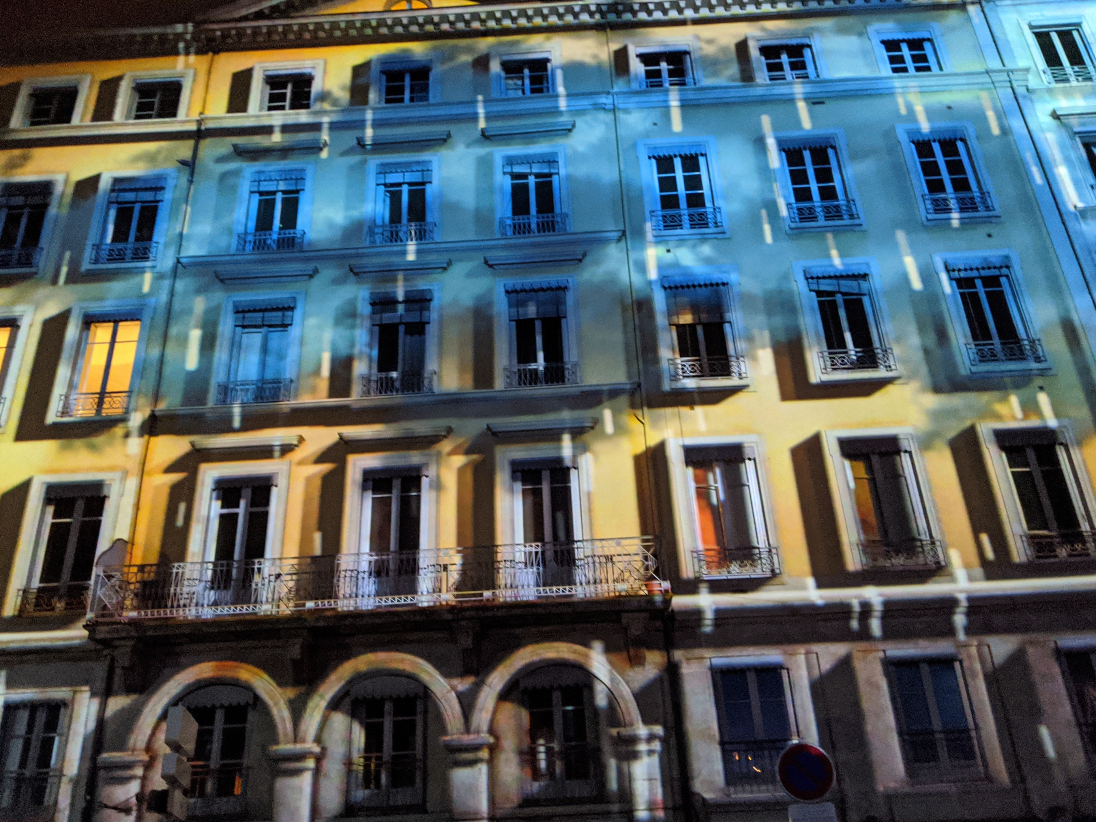
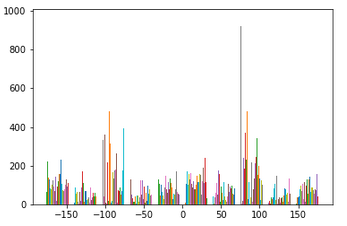
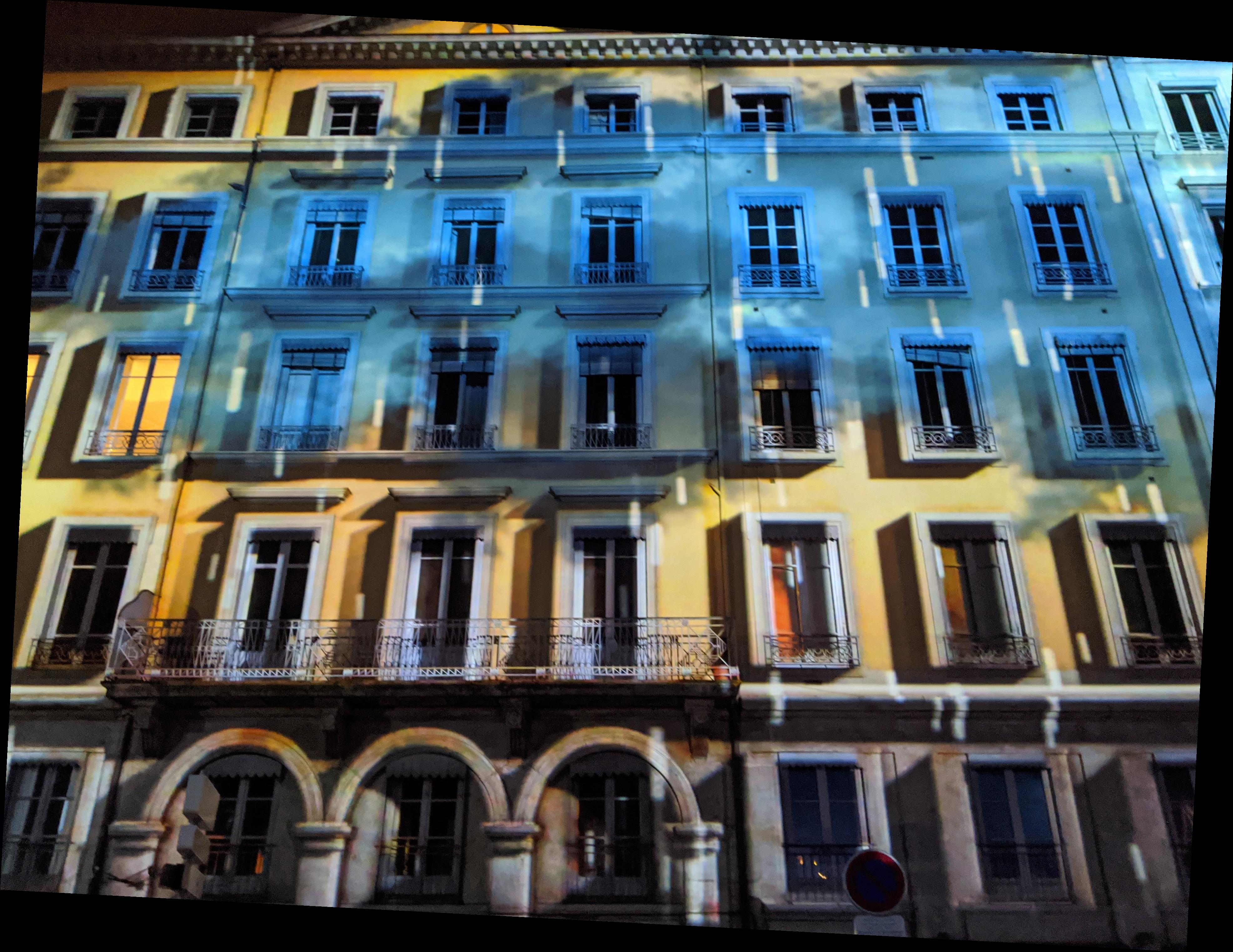
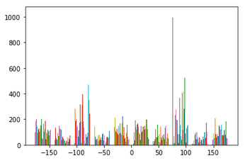
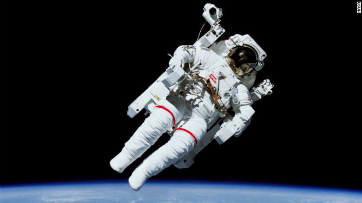
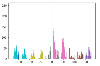
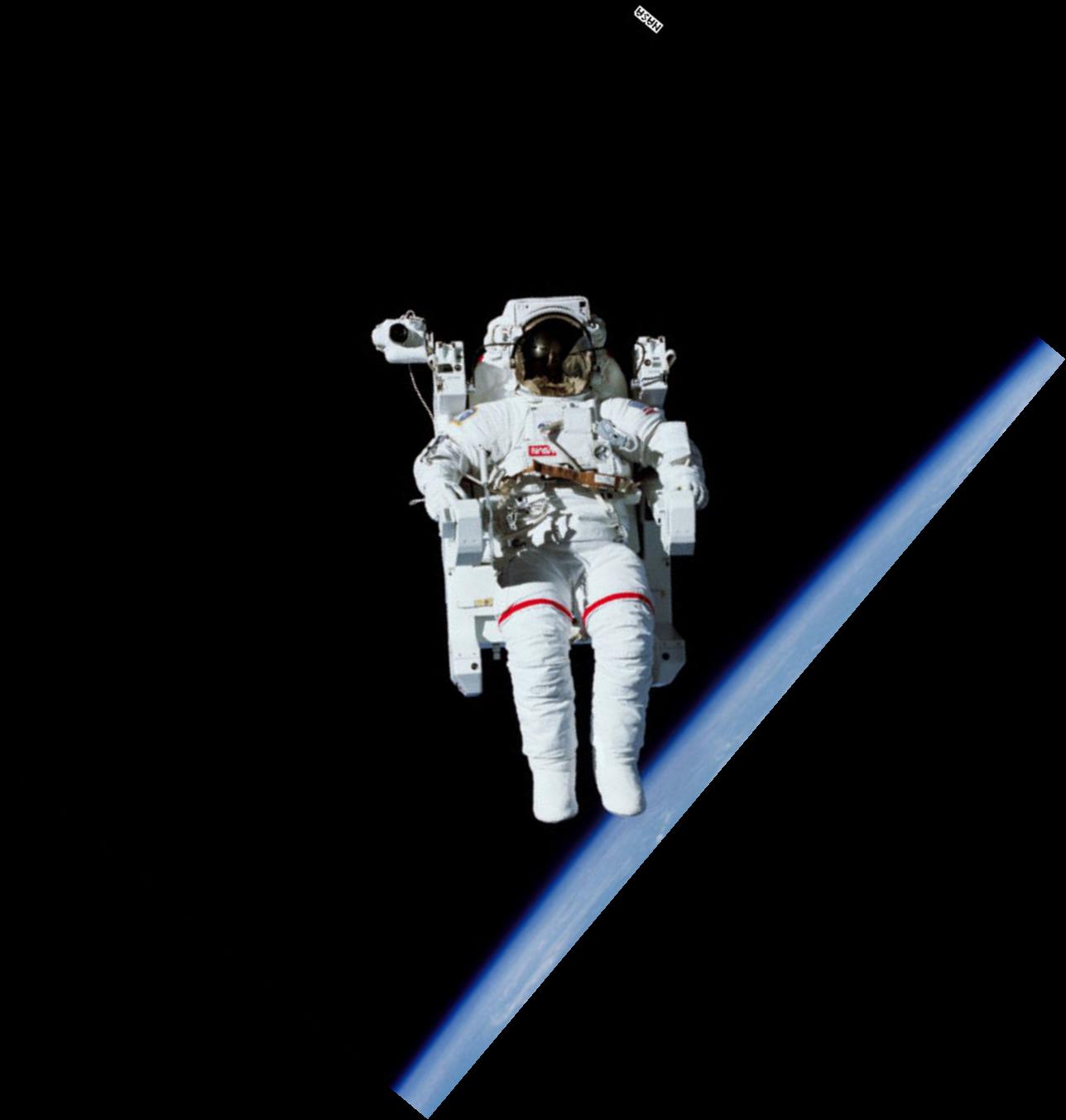
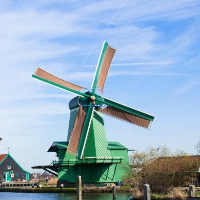
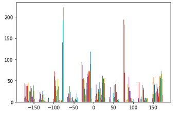
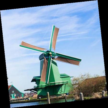
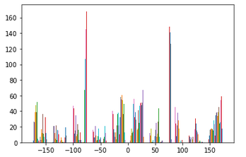
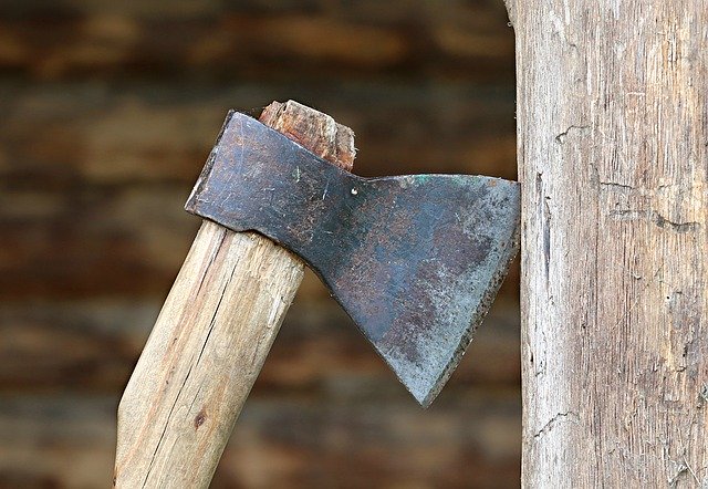
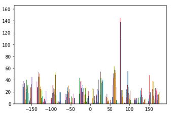
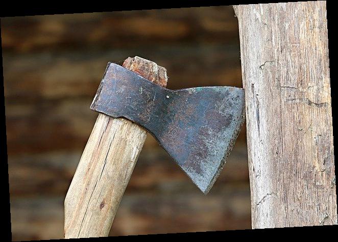
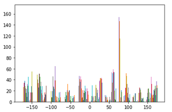
Have you ever stumbled while taking a picture and as a result your image comes out crooked? Well have no fear, because we can straighten your crooked images using gradient angles! The idea in this section is that we will be taking an image that is crooked, calculating various rotations of the image, and scoring the "straightest" rotation. To see how straight a rotation is, we will compute the gradient angle of the edges in the image and see what percentage of the angles fall within -180,-90,0,90, and 180 degrees. The rotation with the highest percentage is the straightest!
|
|
|
|
|
|
|

|
|
|
|
|
|
|
|
|
As you can see, the last two results did not turn out quite how they were expected to. As for the windmill image, even though the blades are diagonal, the base of the building is already fairly straight. Because of this, there was not much rotation needed to "straighten" the image. For the axe image, the whole image was not being accounted for, only the center of the image. Since the center of the image did not have enough information to truly straighten the axe, we see our program returned a failed effort.
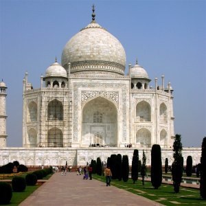
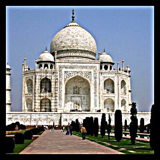
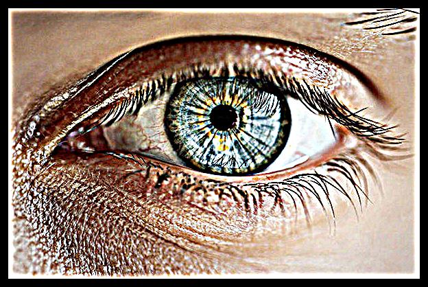
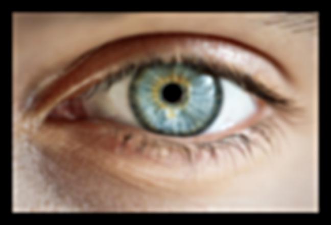
In this section we will be using a special kind of filter called an Unsharp Mask to sharpen images. The idea is that we are going to first find the high frequencies of the image by subtracting the low frequencies. Then we add these high frequencies back to the original image. The results are below.
|
|
|
|
|
|
|
|
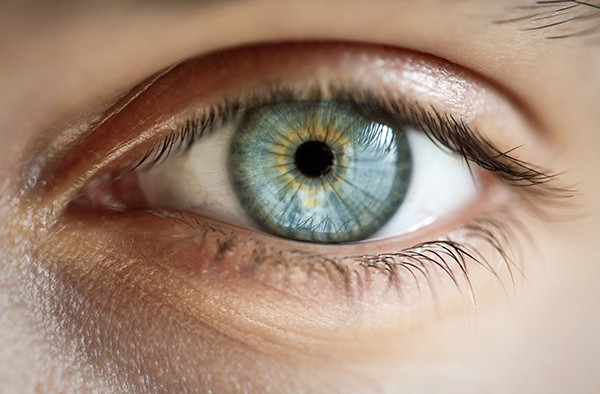
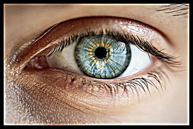
To see the effect of a larger alpha value, note the following image of an eye with alpha = 8. The details are added back in with a much higher intensity.
We will now try to blur an image first and then try sharpening to see what happens. As you will see, we end up with quite a blurry image because our Gaussian blur removed much of the high frequencies that our Unsharp Mask filter relies on for detail.
|
|
|
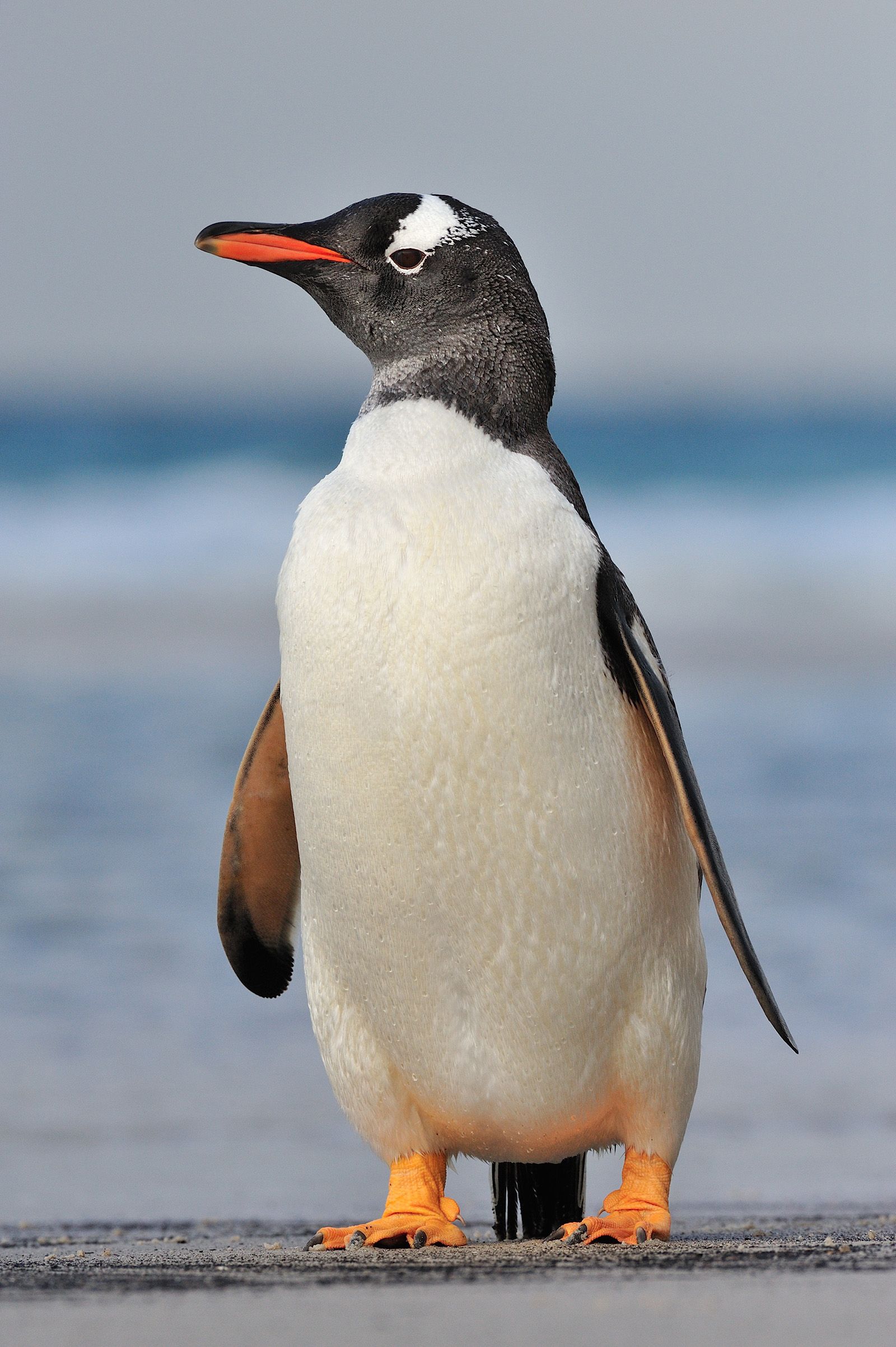
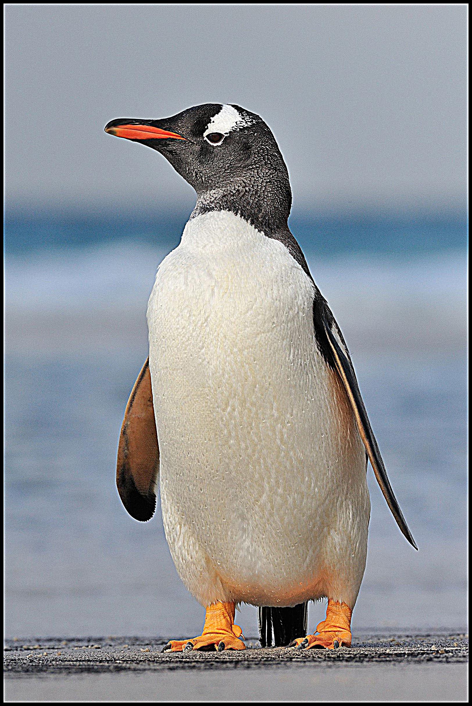
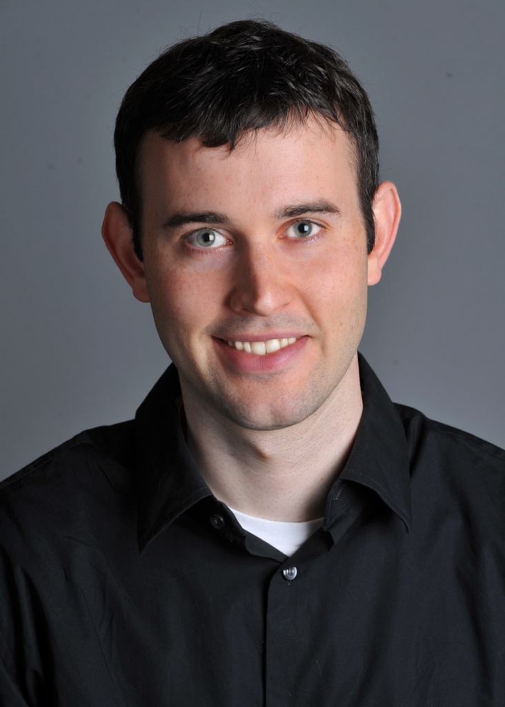
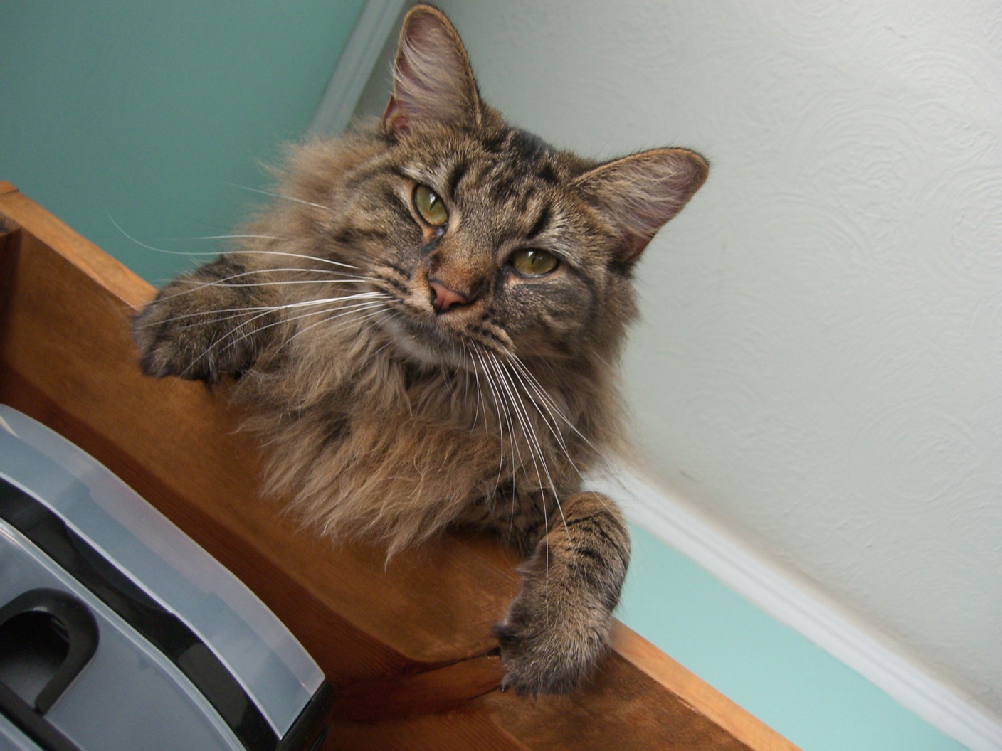
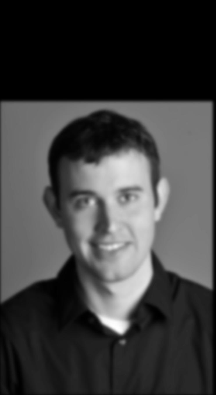
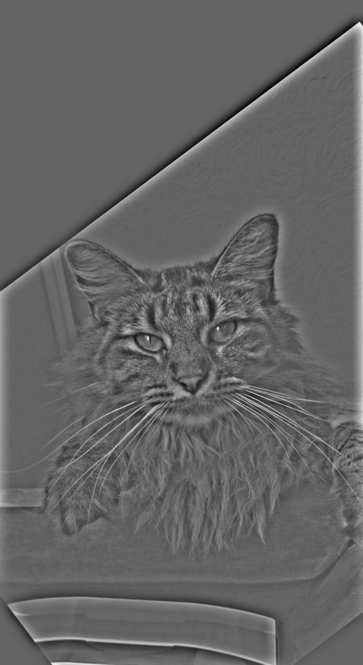
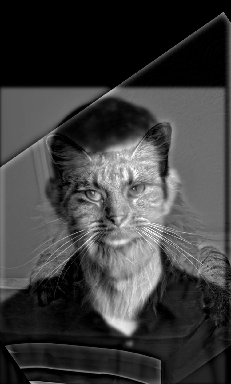
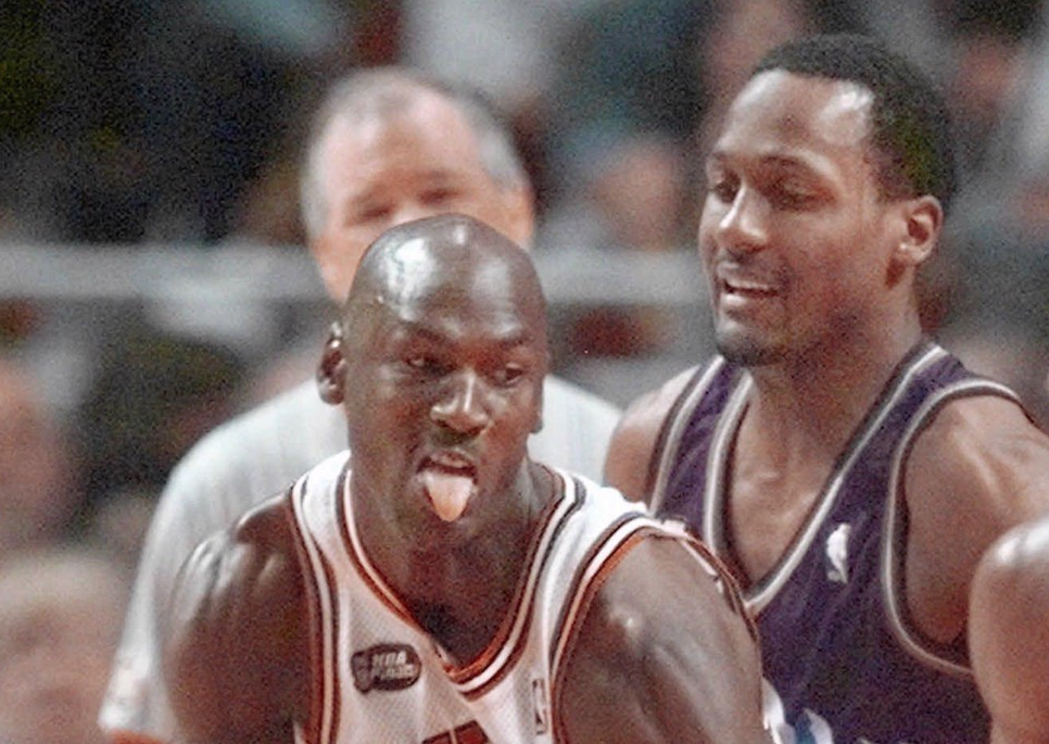
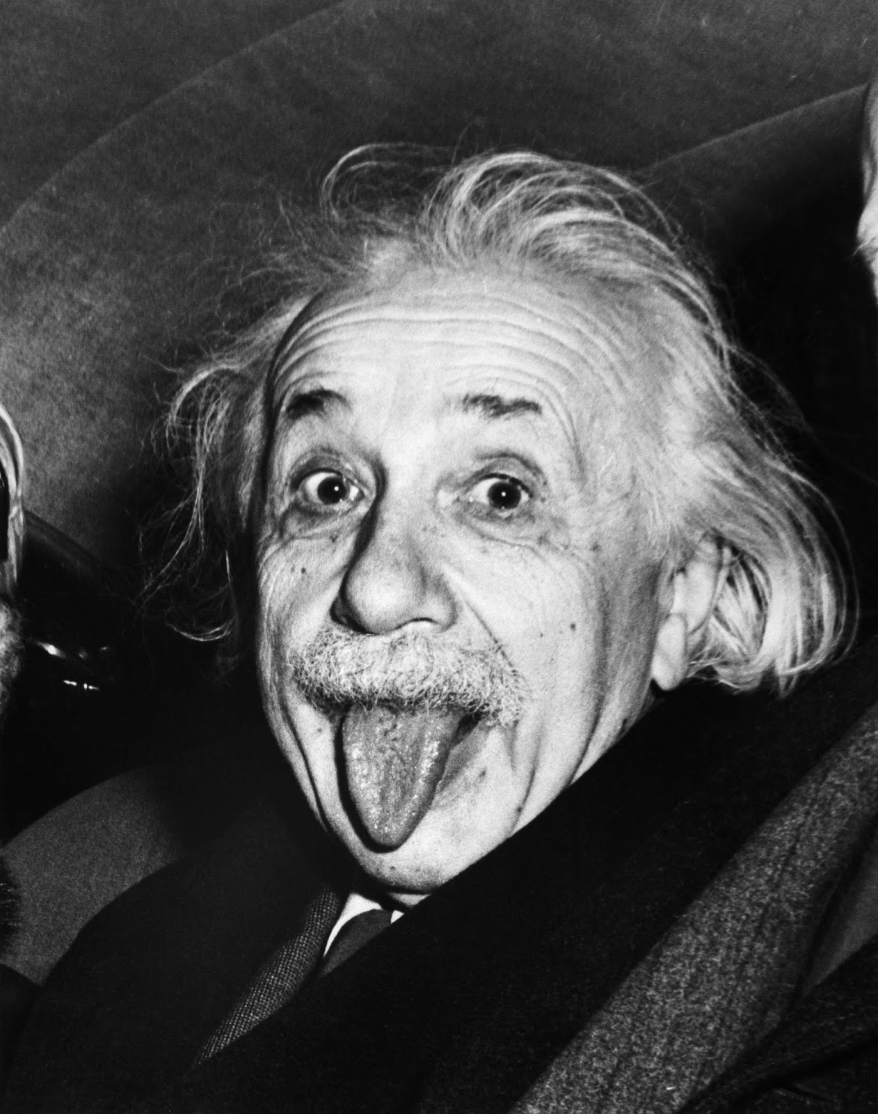
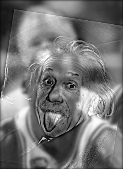
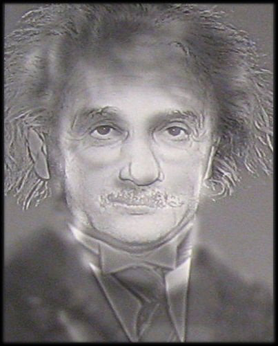
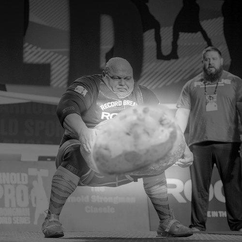
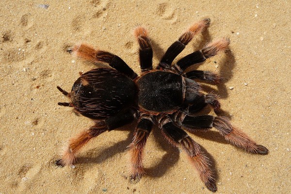
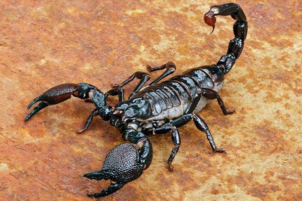
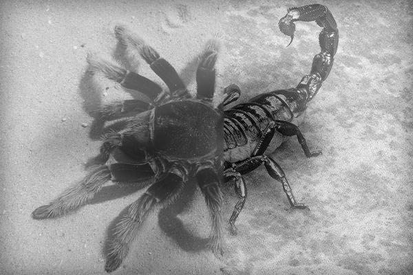
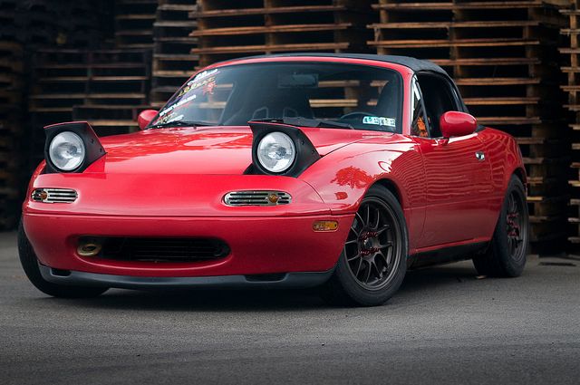
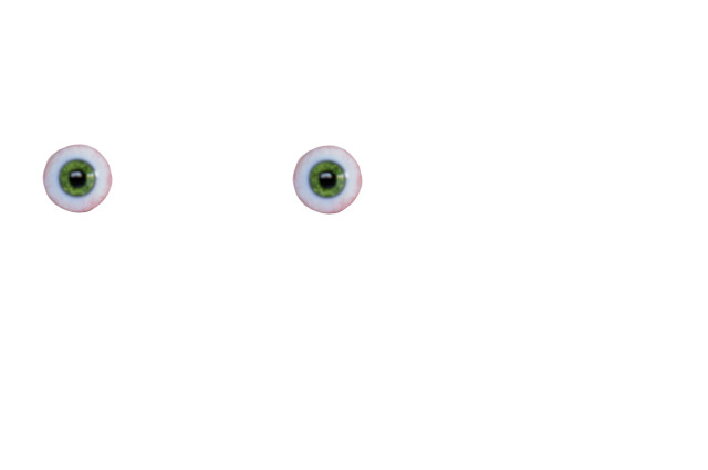
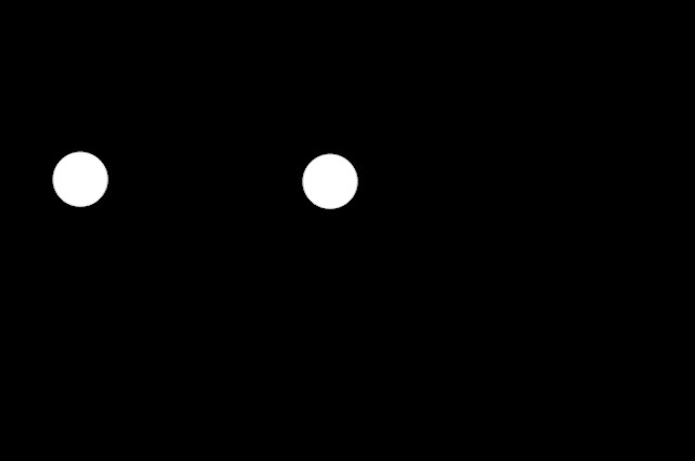
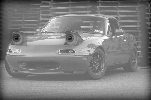
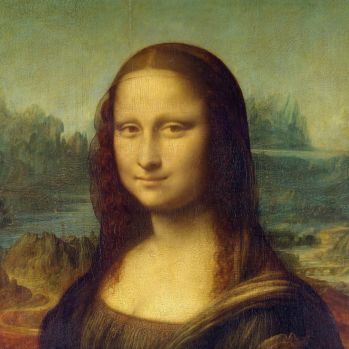
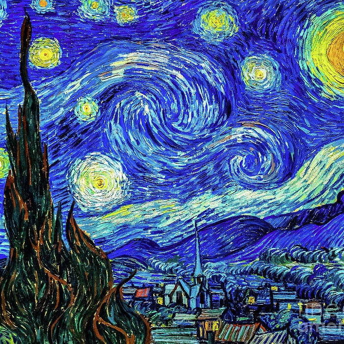
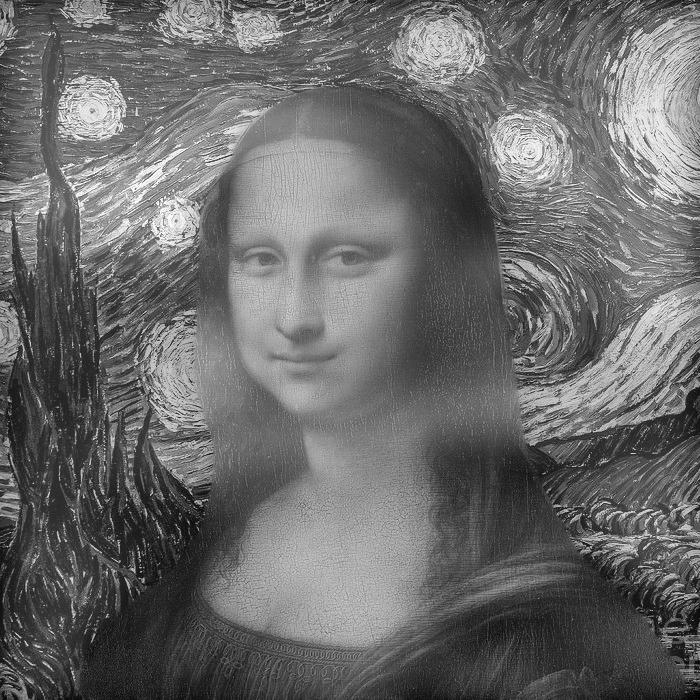
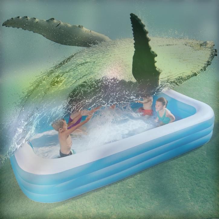
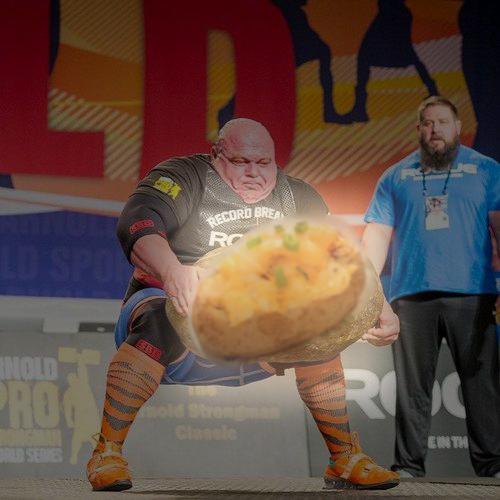
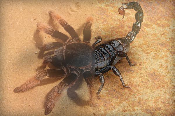
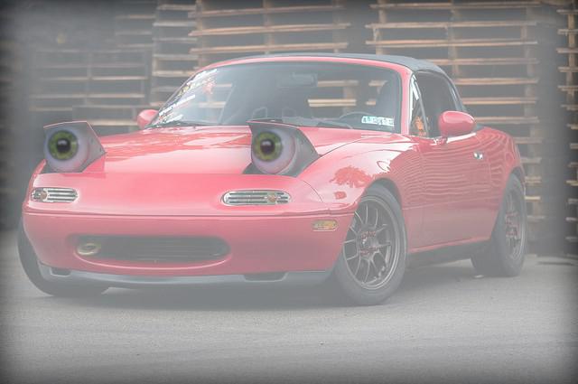
In this section, we will be making hybrid images! This involves aligning two images, isolating their high and low frequencies, and finally stacking the frequencies on top of each other. Up close, we will be able to see the high frequencies of one image, but as we squint our eyes we can see the low frequencies of the second image. Try it out on the images below!
|
| |
|
|
|
|
|
|
|
|
|
|
|
|
|
|
|
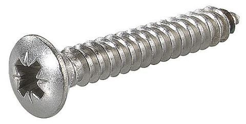
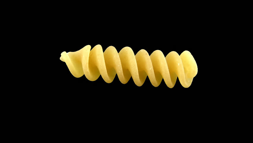
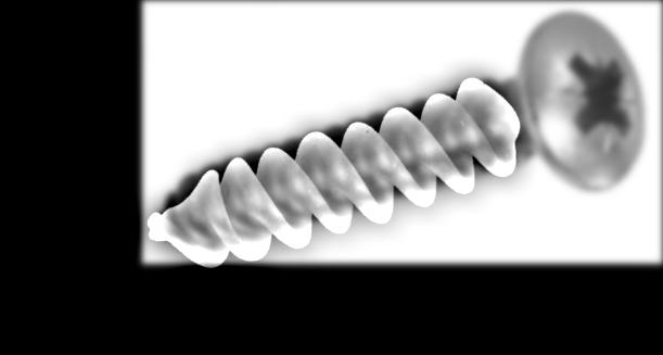
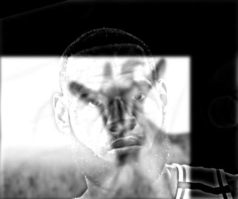
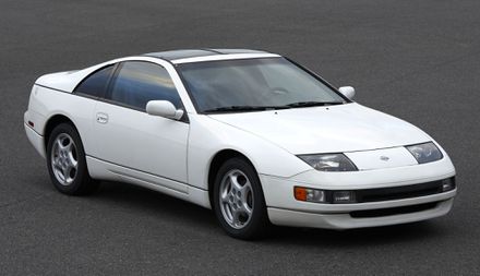
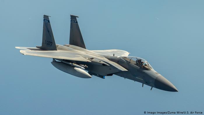
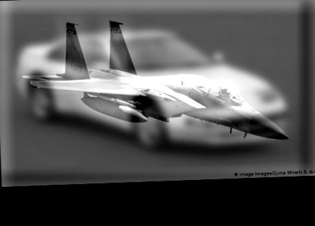
Above, we see the failures that are the JetCar and the FusiScrew. The JetCar failed to produce a convincing result as the two images did not align well in the first place. The FusiScrew is hindered by the cap of the screw that peeks out above the fusili, making it seem like there is only a screw to begin with.
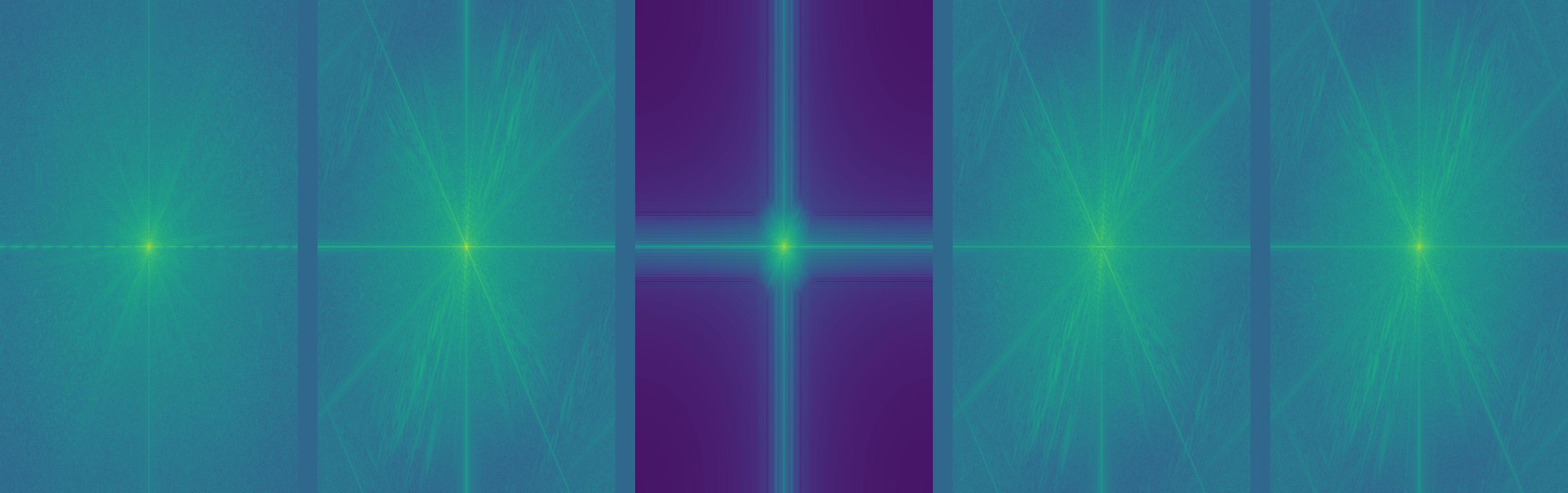
We can also examine the frequency domain of our images above. Let's take a look at the FFT transformations of Nutmeg and Derek. As we will see, our low pass image in the middle completely cuts out all the high frequencies around the center, while our high pass image of nutmeg does the opposite! The FFT of our hybrid image now looks like an addition of our low pass FFT and our high pass FFT!
|
|
|
|
|
|
In this section, we will be observing Gaussian and Laplacian stacks of images. A Gaussian stack is simply an collection of different frequencies of an image. We start with the original image and iteratively apply a Gaussian filter of increasing size/sigma. Every layer represents lower and lower frequencies.
The Laplacian stack is simply the difference between any two layers of our Gaussian stack. Note that our Gaussian stack will contain the original image, but the Laplacian stack will not. We can recreate the original image by adding the last layer of our Gaussian stack to every layer of our Laplacian stack.
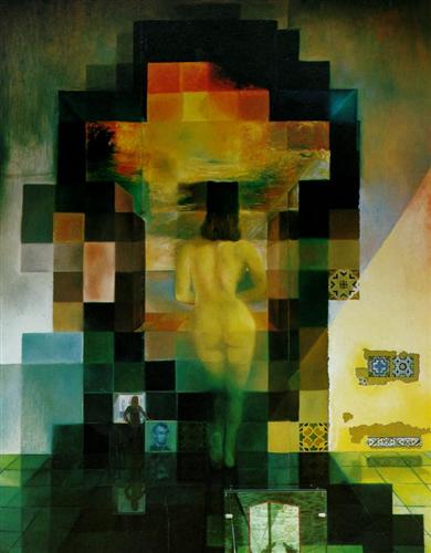
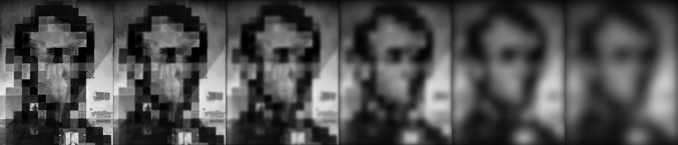
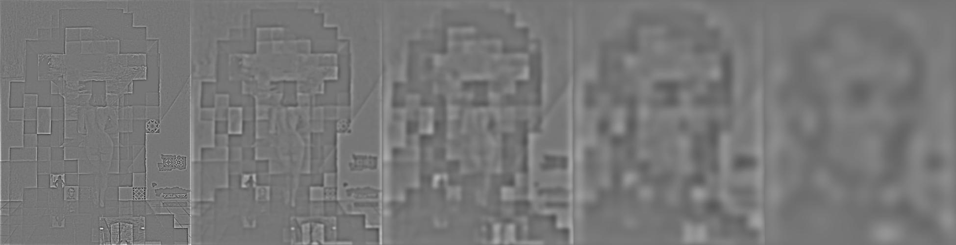
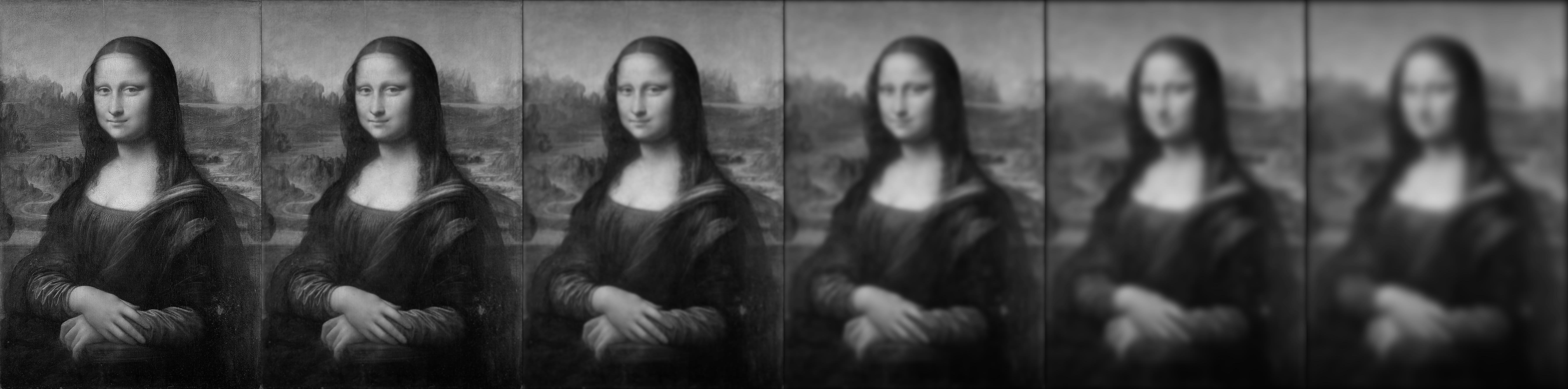
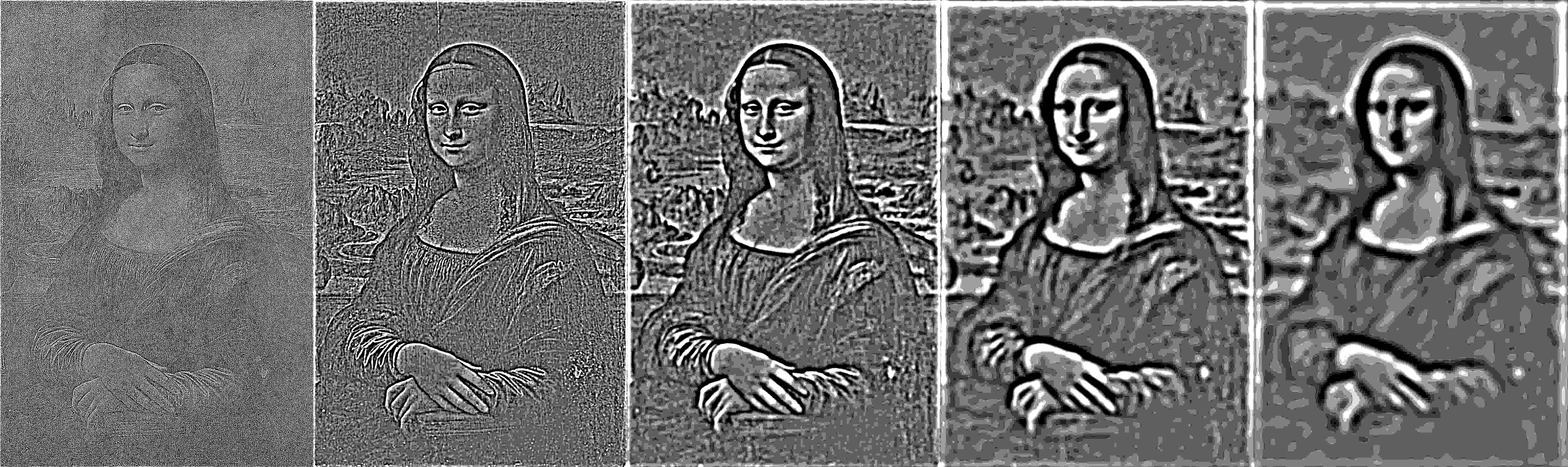
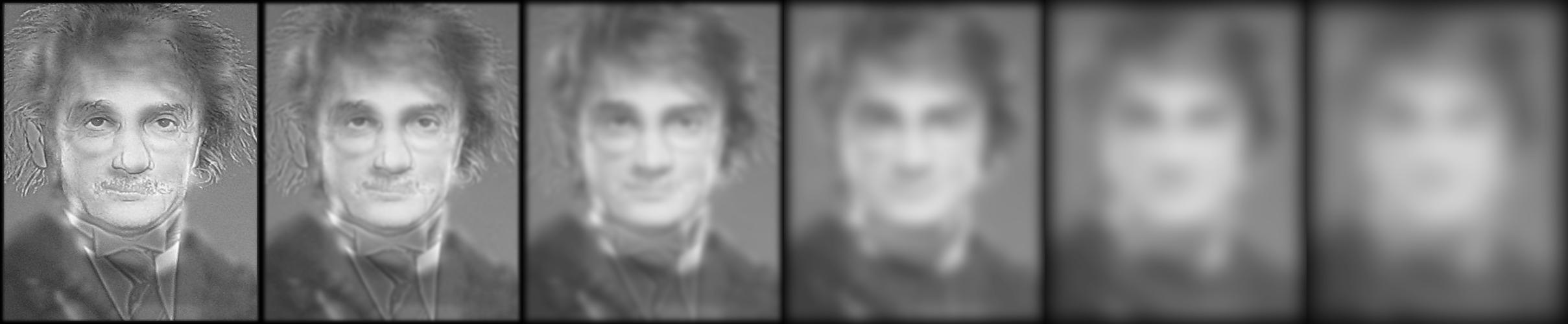
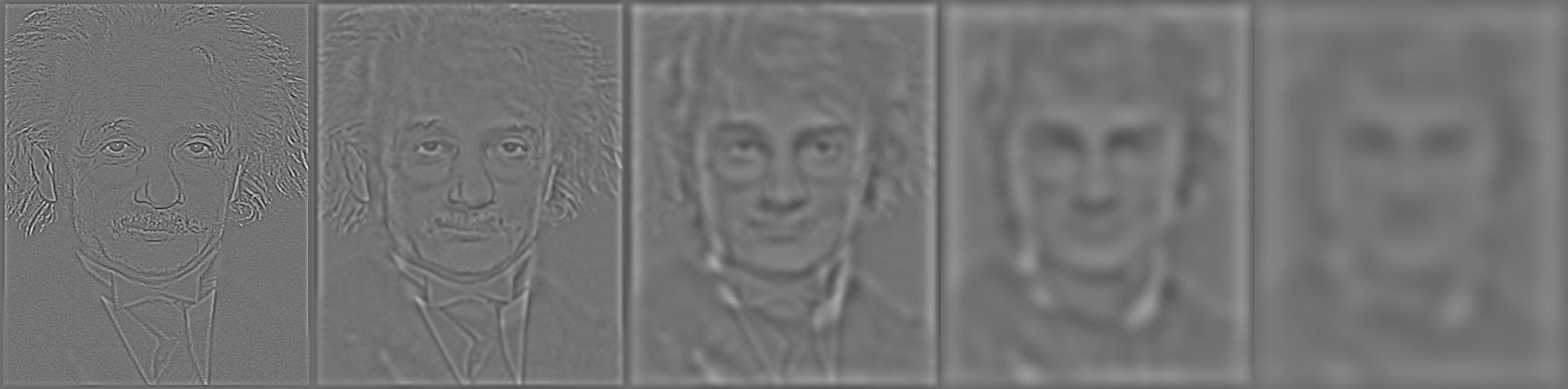
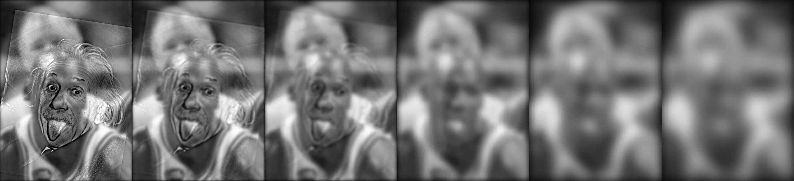
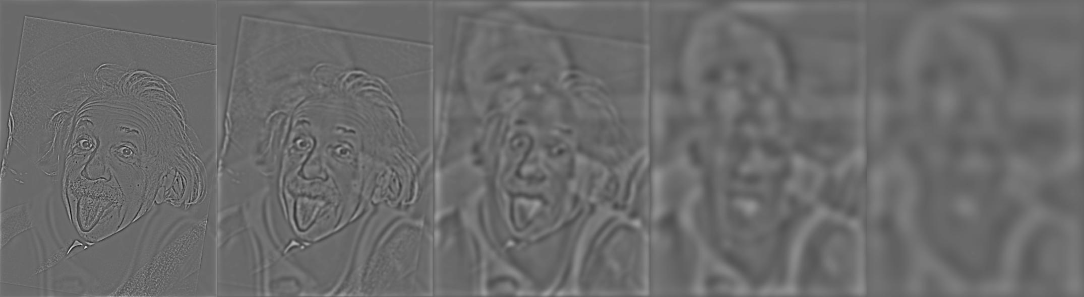
If you look closely through each stack, we can see different images depending on the frequency we are focusing on!
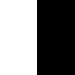
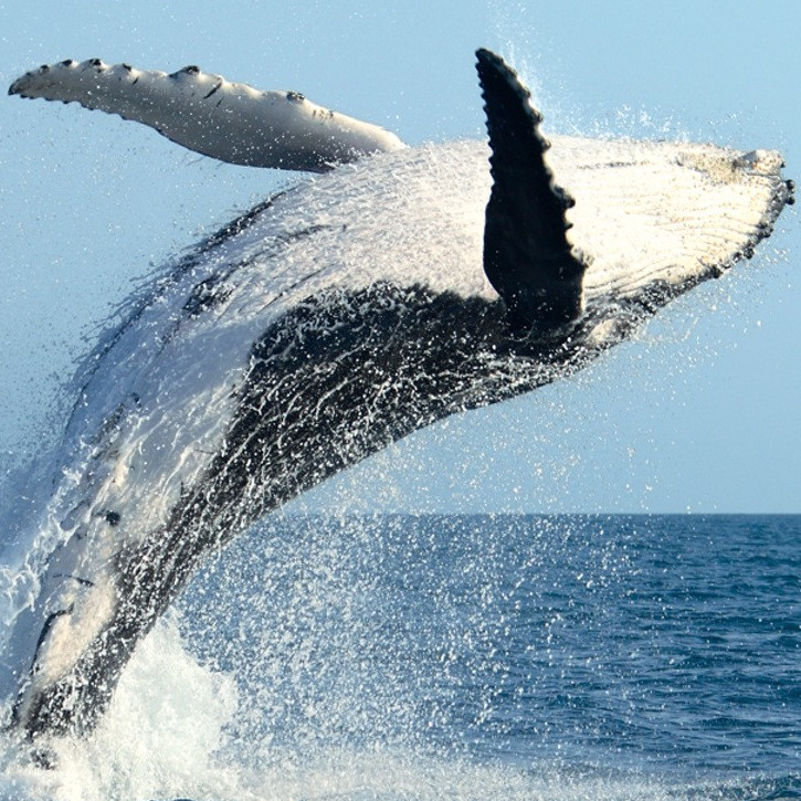
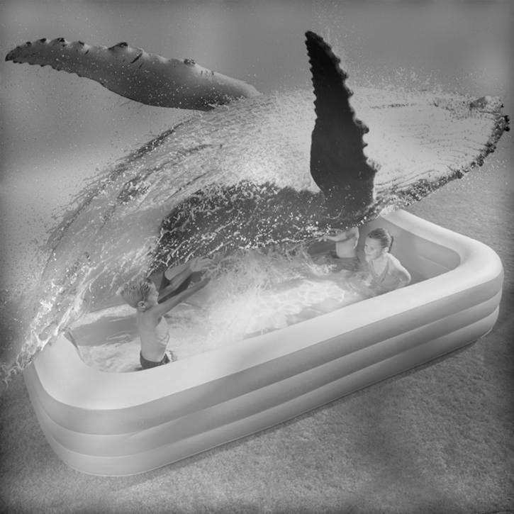
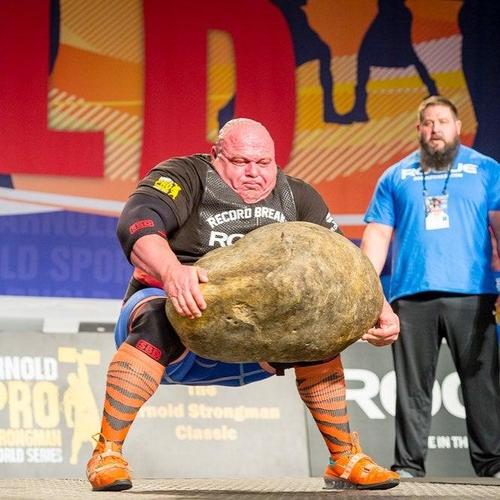
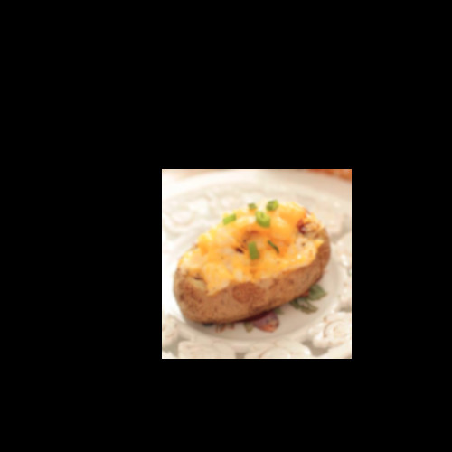
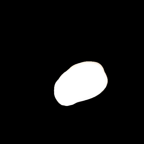
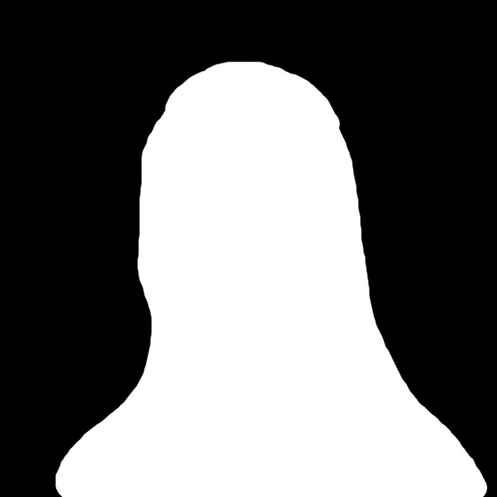
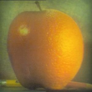
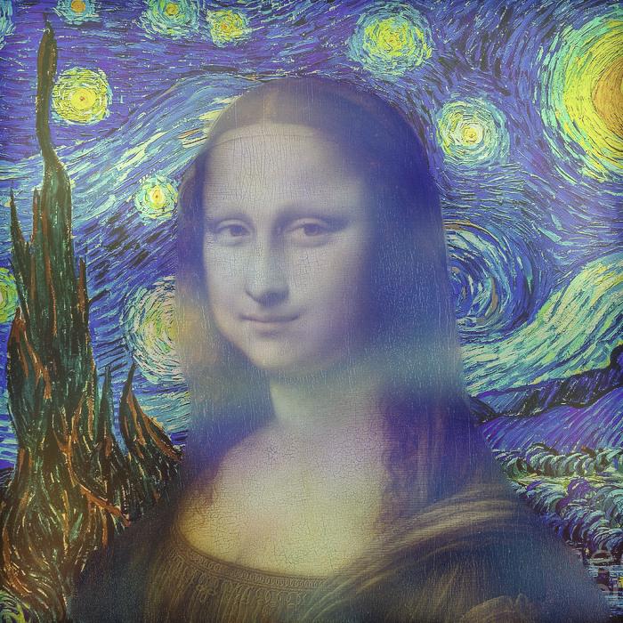
Throughout my entire life I have always dreamed of biting into the mythical apange -- a combination of an apple and an orange. None have ever been seen in person, until now with image blending! In this section we will be blending images using our Gaussian and Laplacian stacks. First, we load two images A and B. We then compute their Laplacian stacks, LA and LB. We also need a mask to indicate where we want our seam between the images. After computing the Gaussian stack of this mask, we calculate the Laplacian stack of our blended image, LS, with the following formula --

Once we have the Laplacian stack of the blended image, we compute sum the last layers of the Gaussian stack for A and B with every layer of LS in order to reconstruct the final blended image!

|

|
|
|
|
|
|
|
|
|
|
|
|
|

|
|
|
|
|
|
|
|
|
|
For bells and whistles I implemented image blending with color! The idea was to treat each color channel as its own image, blend each channel at a time, and join everything together at the end. The results did not turn out as good as I wanted them as they seemed much dimmer than they should be. More time needed to be spent color correcting and making sure darker channel values weren't being clipped. I tried various methods of channel normalization and clipping, but the images still resulted in looking washed out.
|
|
|
|
|
|
|
|
|
|
|
|
|
|
|
|
|
|
|
|
|
|
|
|
|
|
|
|
|
|
Overall, I very much enjoyed this project! I have a better understanding of how altering images in programs like Photoshop works as well as how optical illusions come to be. Also, I now realize just how important filters are in the whole field of image processing! This is the first time I have thought of images as a set of frequences as opposed to a collection of colored pixels.