Part 1.1: Finite Difference Operator
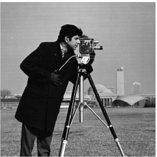
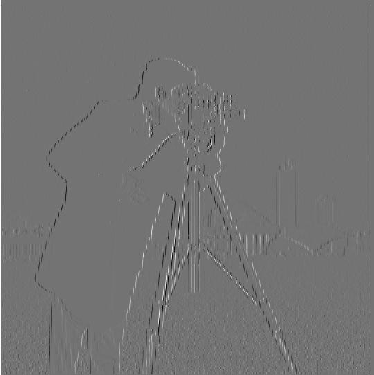
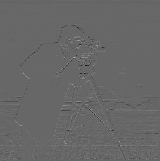
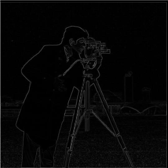
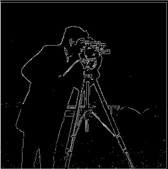
The first part is to play with the basic filter of derivatives in both x and y direction on an original cameraman image. First, I used dx = [1, -1] and dy = [1, -1].T to convolute with the original cameraman photo to get the derivative of x and y. Second, I computed the magnitude of the gradient using the formula np.sqrt(dx^2 + dy^2). Third, I computed the magnitude of the orientaion of the gradient using the formula np.arctan2(-dy, dx). (The grdient is imploved by setting values greater than a certain threshold to 1 and 0 for values under the threshold.)
Part 1.2: Derivative of Gaussian (DoG) Filter
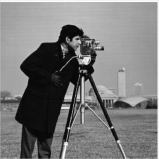
Now we try with the blurred cameraman image below to make it less sharp. in this section I implemented gaussian smoothing to detect the edges and reduce noise. This operation consists of creating a gaussian filter, convolving it with the image, and then convolving the result with the finite difference operators from the previous part. The result is slightly more blurry than the original.
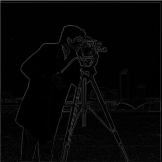
Now we want to apply the gradient mask to this blurry image. Note that we can treat both the gaussian mask and the gradient masks together as a single mask due to the commutative nature of convolution. And here are our new masks(Derivative of Gaussian (DoG))
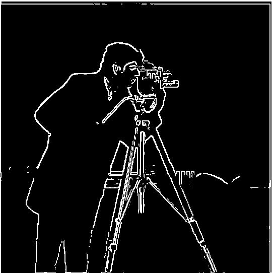
Note that now the gradient magnitude binarized image after DoG looks like a much nice and smoother version of the one before, which is really nice!
Part 1.3: Image Straightening
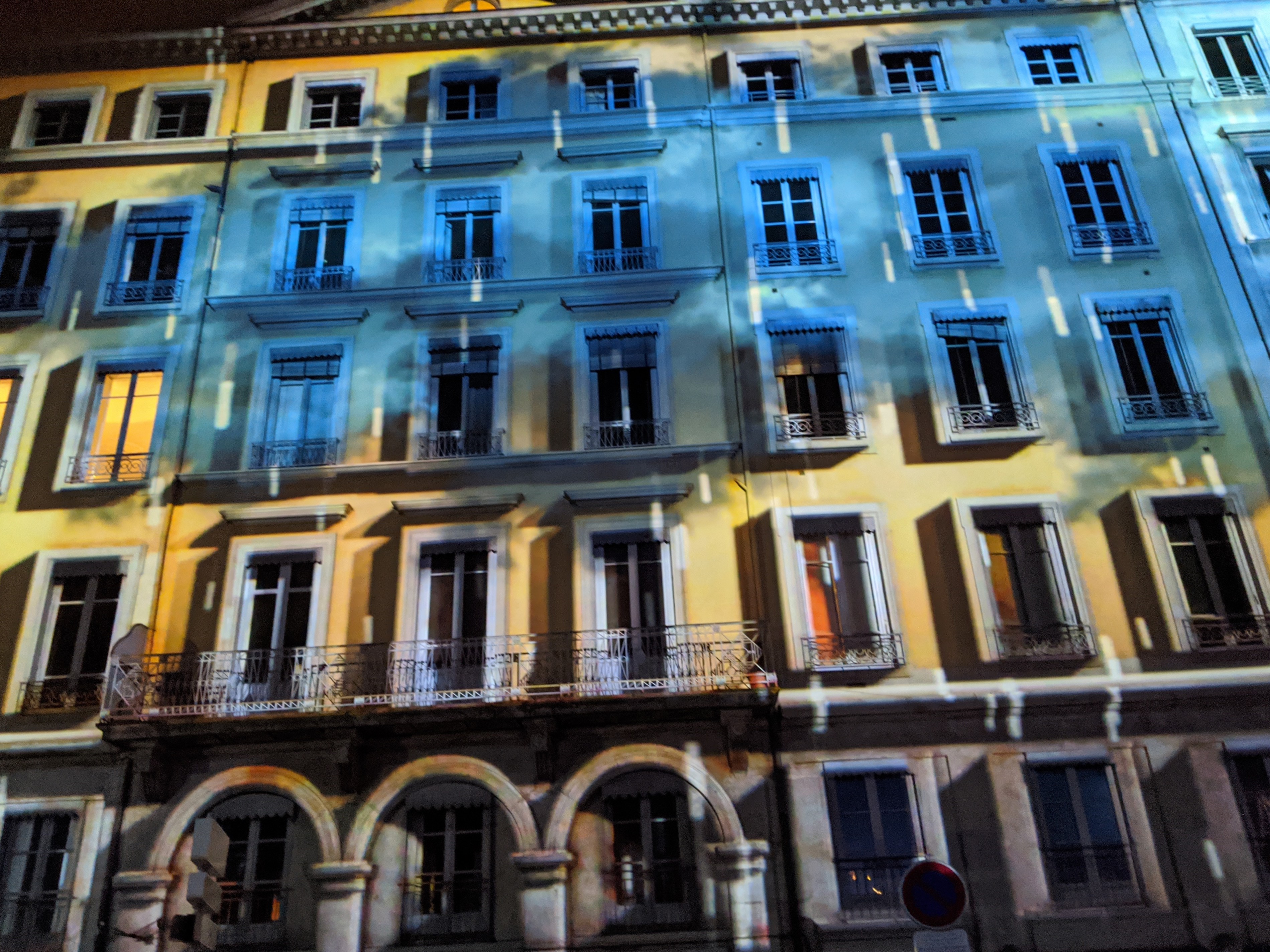
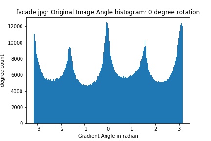
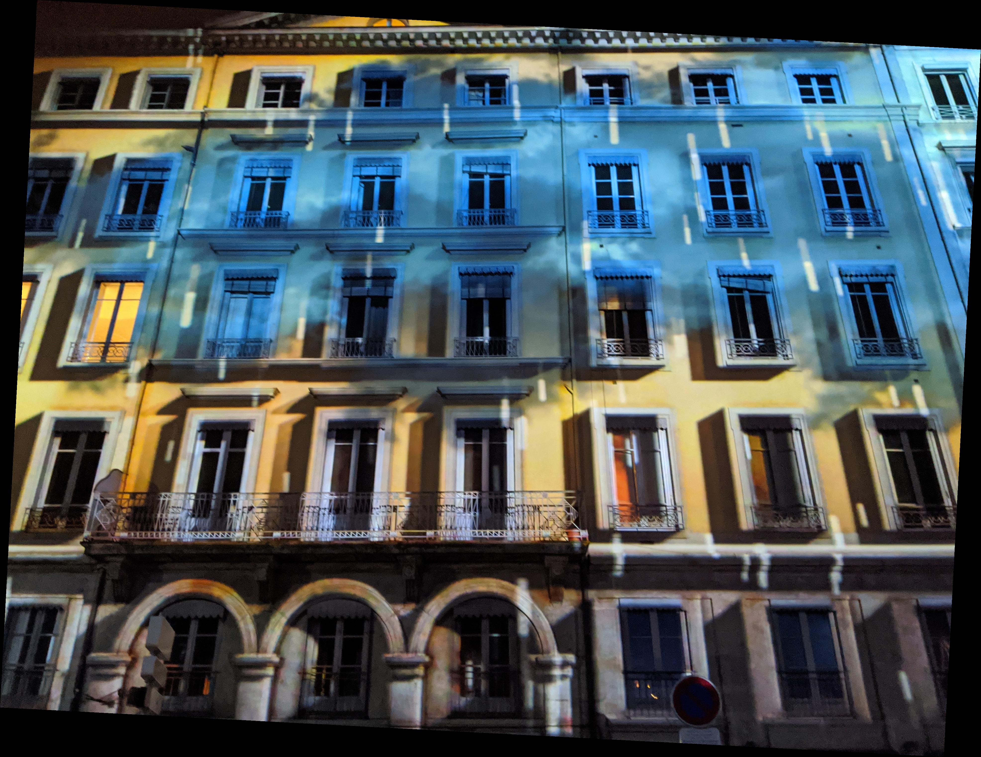
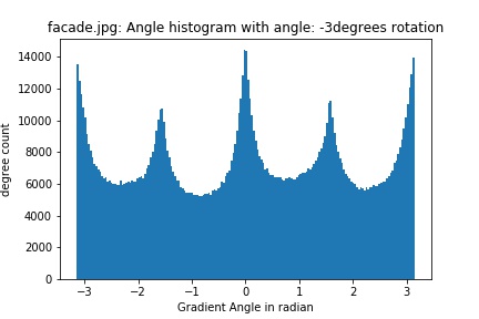
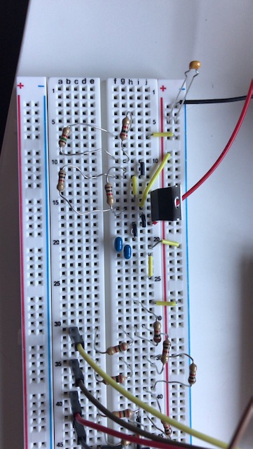
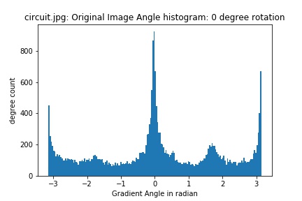
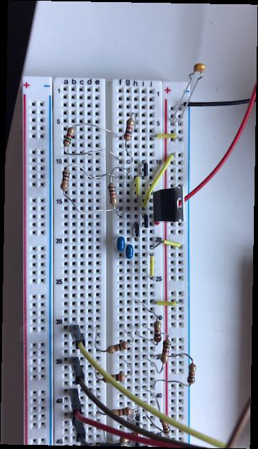
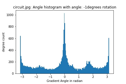
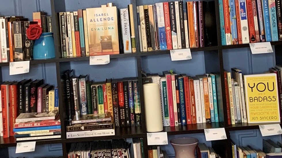
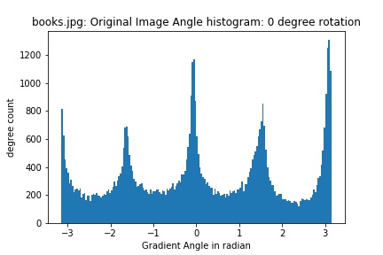
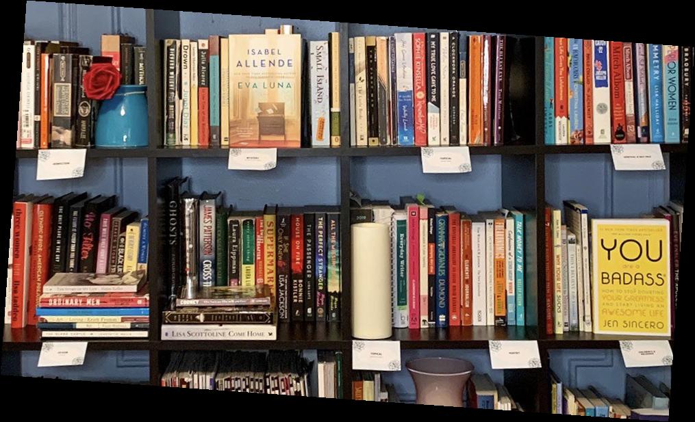
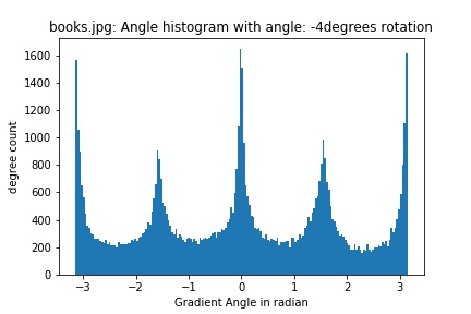
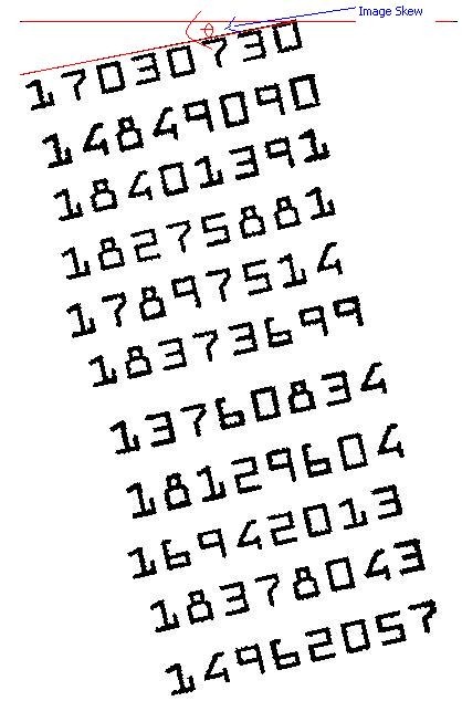
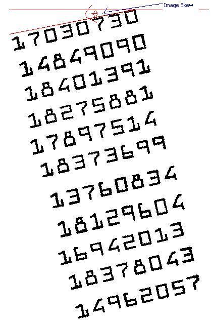
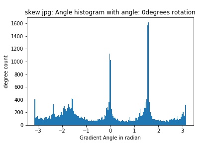
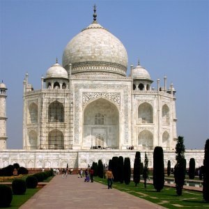
For this part, we would like to take in an image and automatically straighten it. Since most images have a preference for vertical and horizontal edges due to gravity, we essentially want to check whether our edges are close to 0, 90, 180, and 270 degrees. In order to do this, I tested a number of rotations (e.g. from -10 to 10 degrees for facade.jpg)for each image and chose whichever rotation had the maximum count of vertical or horizontal edge pixels. Here are the results and histogram for a number of images:
Now here is one example that fails hugely: this is a skew image of written numbers At first I though this image would be one of the successful examples due to the clear edges between the numbers' dark ink and the white paper. However the result surprises me. In my opinion, one of the reason this fails horribly is that those "edges"(numbers) are not edges by computer's definition. Even in human's eyes they seem to be straight and look like edges, from a lower resolution, they are very just curly thick black lines that have nothing to do with straightening edges. And I believe one of the ways to improve it might be using the Fourier domain.
Part 2.1: Image "Sharpening"
In this portion of the project, we are sharpening images by adding the image's high frequency elements to its original image. Remember in part 1.2, we have Gaussian filter (g), as known as the low-pass filter. Naturally, if f is our original image, f * g is our blurred or image with lower frequencies and f - (f * g) would be our image with higher frequencies elements. If we can intensify these high frequencies elements (by adding them back to the original image), we have a sharper image! These operations can be combined into a single convolution operation called the unsharp mask filter: f + a(f - f * g) = f * ((1 + a)e - ag), where e is the identity filter.
here we present another interesting example. Below on the left is a image with very high resolution (very sharp already). We first blur this original image by using Gaussian filter(result is the middle image). Next we tried to re-sharpen this blurred version (the image on the right). Note that even though the resharpened version is better than the blurred one, there is a huge discrepancy between it and the original. This is due to the fact that this method is actually a deception: there is no additional information added, but rather only a manipulation of the already known high frequencies elements. However, the blurry process (Gaussian filter in this case) always loses some information. And the end result is the discrepancy between the two images.(The difference is hard to see, you may need to zoom in.)
Part 2.2: Hybrid Images
Motivation: The goal of this part of the assignment is to create hybrid images using the approach described in the SIGGRAPH 2006 paper by Oliva, Torralba, and Schyns. Hybrid images are static images that change in interpretation as a function of the viewing distance. The basic idea is that high frequency tends to dominate perception when it is available, but, at a distance, only the low frequency (smooth) part of the signal can be seen.
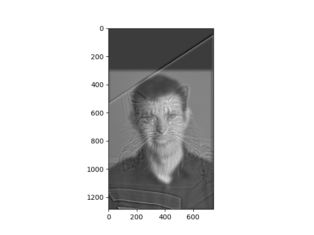
In this part, the goal is to use two images(after aligning them and cropping them) to create a hybrid image. The idea is that we only keep the low frequency elements of one image and the high frequency elements of the other image. The combined result would be a very interesting image that tricks our mind if observed from a different distance.
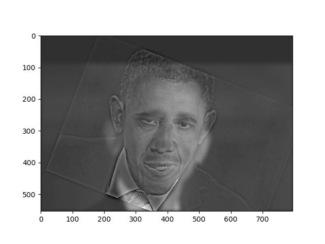
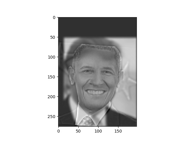
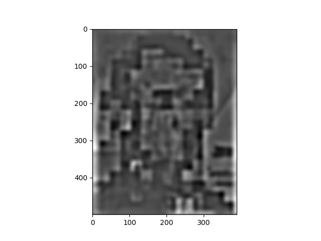
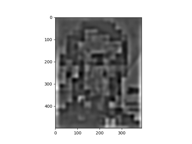
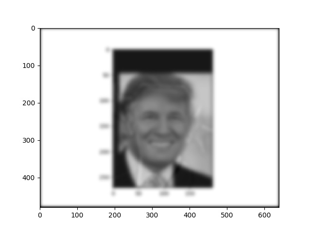
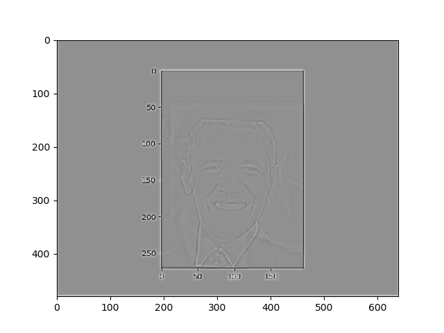
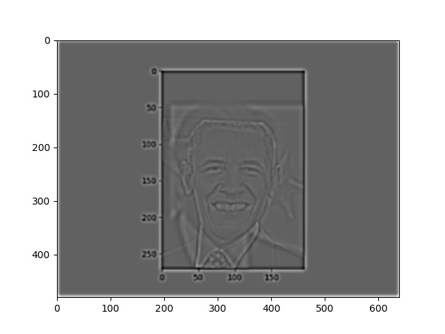
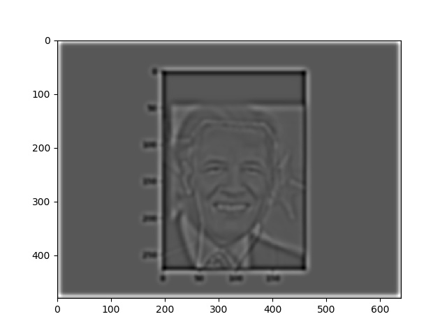
here we present a failed example. In this exmaple, no matter how close you are to the image, it is really hard to see th facial expression of president Obama. He looks angry from his mouth, but he also looks funny from his eyebrows. I would consider this as a failed example becasue even though we can clearly see the smily Obama from a far distance, it is ambiguous to find the proper image from a close distance.
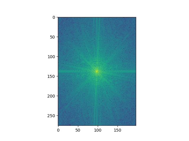
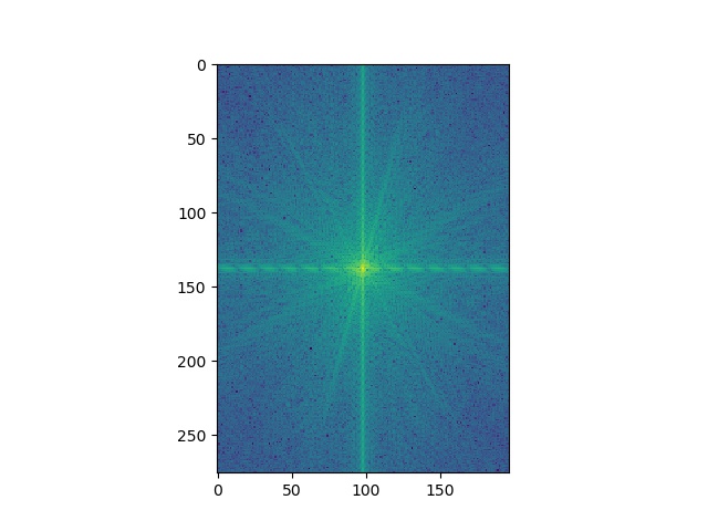
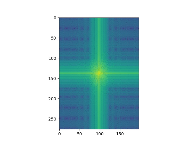
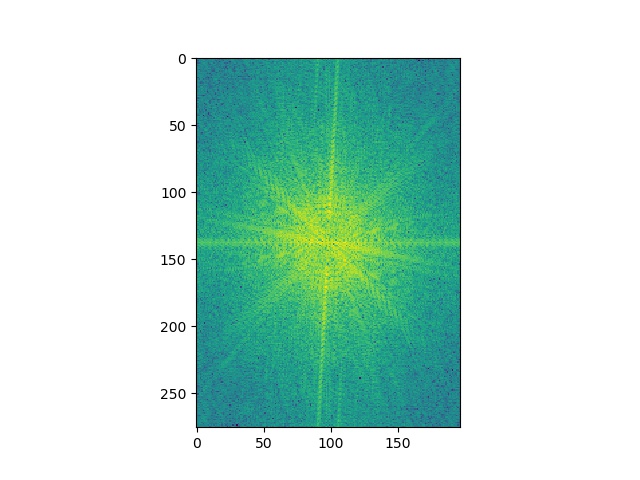
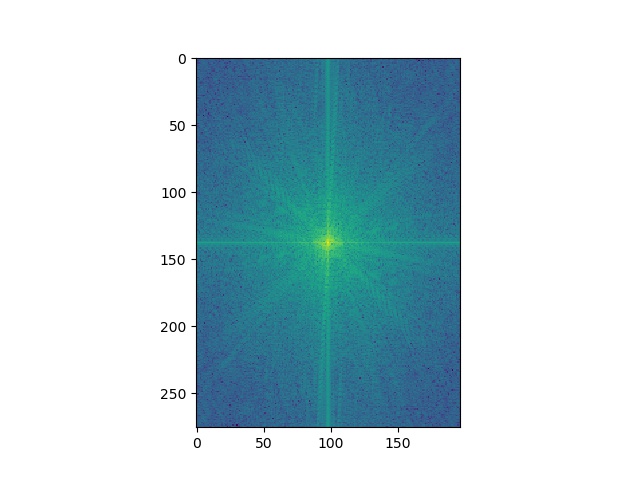
For the the above set of images, I displayed the images in the log Fourier domain. The highpass Fourier image can be seen to have more high frequencies due to the spread of the points while the lowpass Fourier image points are more centered around the middle.
Part 2.3: Gaussian and Laplacian Stacks
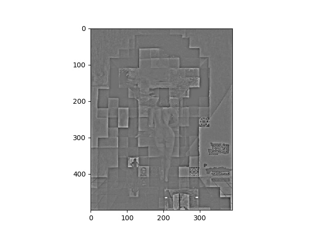
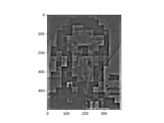
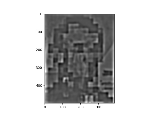
In this part I implement Gaussian and Laplacian stacks. The Gaussian stack was created by repeatedly applying a gaussian filter to the previous image on the stack. The Laplacian stack was created by subtracting the neighboring images in the Gaussian stack. In my examples below, the first row here is the Gaussian stack and the second row is the Laplacian stack.
Part 2.4: Multiresolution Blending (a.k.a. the oraple!)
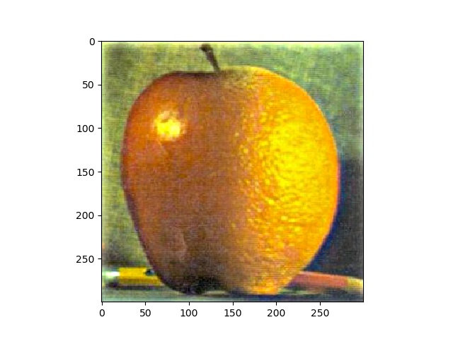
The goal of this part of the assignment is to blend two images seamlessly using a multi resolution blending as described in the 1983 paper by Burt and Adelson. An image spline is a smooth seam joining two image together by gently distorting them. Multiresolution blending computes a gentle seam between the two images seperately at each band of image frequencies, resulting in a much smoother seam
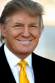
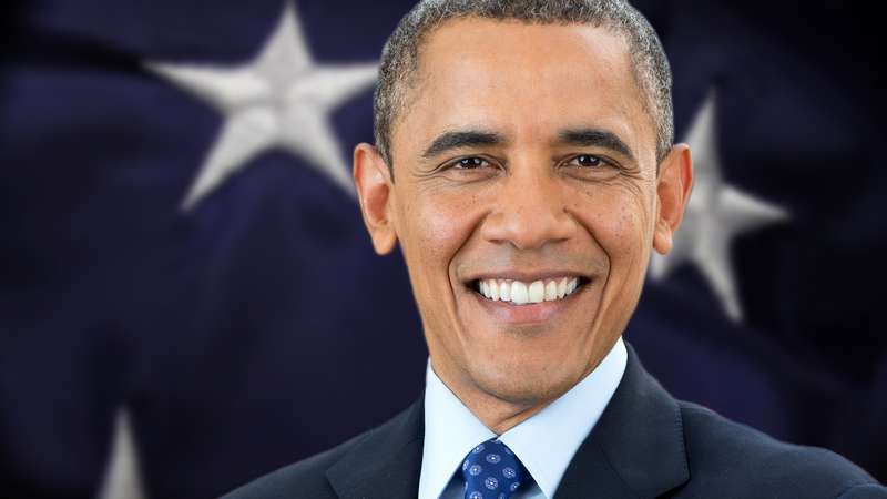
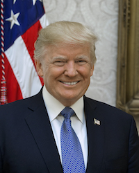
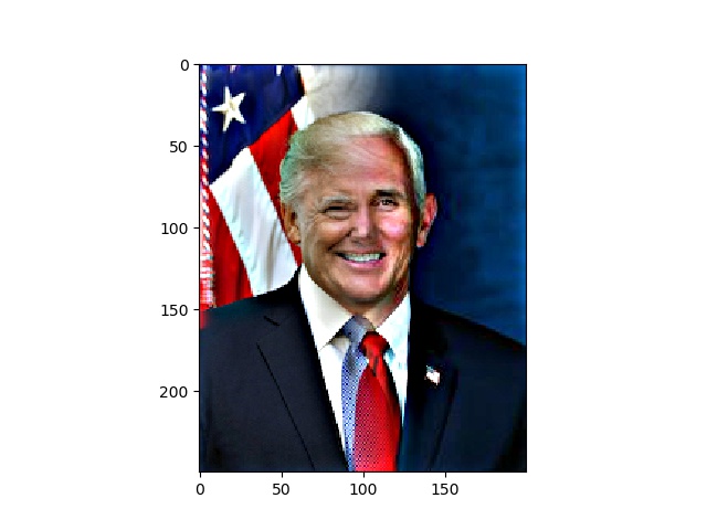
Below is another blending example with two human images. Note that this is harder than the previous example due to the fact that there are many elements in the picture that are hard to be aligned with.
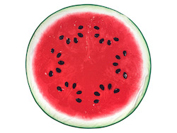
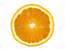
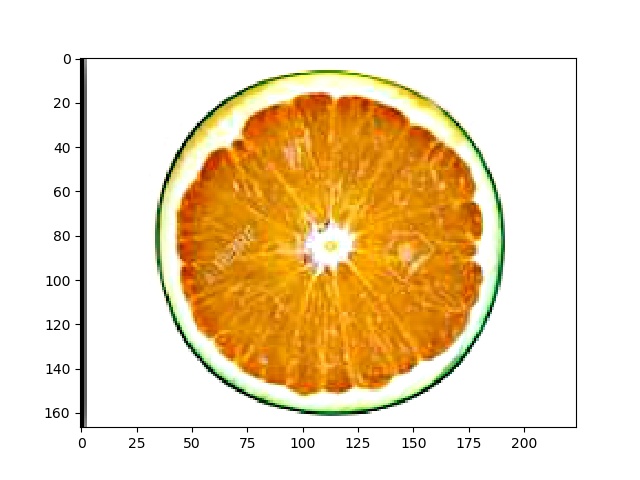
Below is a blending example with a non-linear mask: this time it is a circular mask that changes a watermelon into a orangemelon!
