import numpy as np
import skimage as sk
import skimage.io as skio
import skimage.transform
import skimage.color as sc
import time

from scipy.signal import convolve2d
from scipy.signal import convolve
from scipy.ndimage.interpolation import rotate
import cv2

import seaborn as sns
import matplotlib.pyplot as plt

import warnings
warnings.filterwarnings('ignore')
Project 2: Fun with Filters and Frequencies!
David Yi
Part 1: Fun with Filters
Part 1.1: Finite Difference Operator
In the first section, we use the finite difference operators to generate derivative images, compute the gradient magnitude image, and apply a binary threshold mask to find the edges of the image. We find the gradient magnitude image by finding the magnitude of the sum of our squared derivative matrices.
$ M = \sqrt{(dx^2 + dy^2)}$
cman = skio.imread('cameraman.png')
cgray = sc.rgb2gray(cman)
D_x = np.array([[1, -1],
                 [0, 0]])
D_y = np.array([[1, 0],
                [-1, 0]])
Image of Camera Man
skio.imshow(cgray);

cd_x = convolve2d(cgray, D_x)
cd_y = convolve2d(cgray, D_y)
# Gradient Magnitude Image
c_gradient = np.sqrt(cd_x**2 + cd_y**2)
# plt.title('dx image')
# plt.imshow(cd_x, cmap='gray')
# plt.axis('off')
# plt.imsave('cd_x.jpg', cd_x, cmap='gray')

# plt.title('dy image')
# plt.imshow(cd_y, cmap='gray')
# plt.axis('off');
# plt.imsave('cd_y.jpg', c_gradient, cmap='gray')

# plt.title('gradient magnitude image')
# plt.imshow(c_gradient, cmap='gray')
# plt.axis('off');
# plt.imsave('cd_gradient.jpg', c_gradient, cmap='gray')
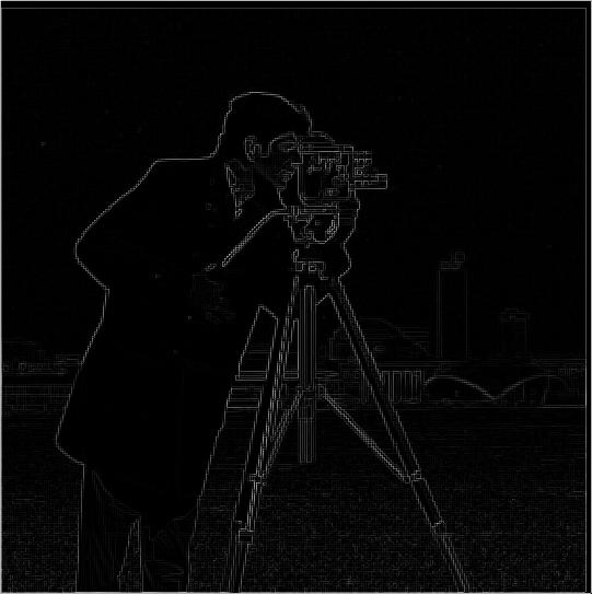
dx filter (left), dy filter (middle), gradient magnitudes (right)
 |
 |
 |
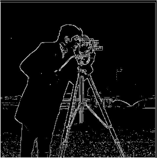
With a threshold of 0.15, the edges of our image are extremely noisy, especially with the water pixels around the bottom:
# Threshold of 0.05 to suppress noise while still detecting borders
skio.imshow((c_gradient>0.15));
plt.imsave('thresh.jpg', (c_gradient>0.15), cmap='gray')
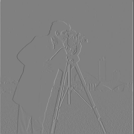
1.2 Derivative of Gaussian (DoG) Filter
Our results from 1.1 hint that a simple derivative filter is not enough to detect the edges of our image. In this section, we smooth our image with gaussian filter to remove noise before convoluting with the finite difference vectors.
#
g_1d = cv2.getGaussianKernel(ksize=6, sigma=2)
g_2d = g_1d @ g_1d.T
# Apply Gaussian Smoothing to image and convolve smoothed image with finite difference vectors
cam_smoothed = convolve2d(cgray, g_2d)
cam_smooth_x = convolve2d(cam_smoothed, D_x)
cam_smooth_y = convolve2d(cam_smoothed, D_y)
c_smooth_gradient = np.sqrt(cam_smooth_x**2 + cam_smooth_y**2)
With Gaussian Smoothing
# plt.title('smooth dx image')
# plt.imshow(cam_smooth_x, cmap='gray')
# plt.axis('off')
# plt.imsave('scd_x.jpg', cd_x, cmap='gray')

# plt.title('smooth dy image')
# plt.imshow(cam_smooth_y, cmap='gray')
# plt.axis('off');
# plt.imsave('scd_y.jpg', c_gradient, cmap='gray')

# plt.title('smooth gradient magnitude image')
# plt.imshow(c_smooth_gradient, cmap='gray')
# plt.axis('off');
# plt.imsave('scd_gradient.jpg', c_gradient, cmap='gray')
dx filter (left), dy filter (middle), gradient magnitudes (right)
 |
 |
 |
# skio.imshow((c_smooth_gradient>0.05));
# plt.imsave('c_smooth.jpg', (c_smooth_gradient>0.05), cmap='gray')
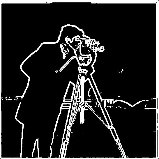
After applying gaussian smoothing to the image with a threshold of 0.05, we see that the edges are much bolder and less noisy (especially around the bottom with the water pixels). We are also able to maintain difficult edges like the tall building in the back by setting a low threshold value without the image being too blurry.
Derivative of Gaussian Filter
We can achieve the same solution by convolving the gaussian filter with the finite difference vectors before convolving with our original image to save computation time. Below, we verify that we get the same result.
gauss_dx = convolve2d(g_2d, D_x)
gauss_dy = convolve2d(g_2d, D_y)
man_gauss_dx = convolve2d(cgray, gauss_dx)
man_gauss_dy = convolve2d(cgray, gauss_dy)
plt.imshow(gauss_dx, cmap='gray')
plt.axis('off')
plt.imsave('gauss_x.jpg', gauss_dx, cmap='gray')

plt.imshow(gauss_dy, cmap='gray')
plt.axis('off');
plt.imsave('gauss_y.jpg', gauss_dy, cmap='gray')

plt.imshow(man_gauss_dx, cmap='gray')
plt.axis('off');
plt.imsave('man_gauss_dx.jpg', man_gauss_dx, cmap='gray')

plt.imshow(man_gauss_dy, cmap='gray')
plt.axis('off');
plt.imsave('man_gauss_dy.jpg', man_gauss_dx, cmap='gray')

skio.imshow(gauss_dx)

skio.imshow(gauss_dy)

Derivative of Gaussian (dx) and Derivative of Gaussian (dy)
plt.subplot(1, 2, 1)
skio.imshow(gauss_dx)

plt.subplot(1, 2, 2)
skio.imshow(gauss_dy);

Convolution with Derivative of dx and dy Gaussians
 |
 |
# c_gauss_gradient = np.sqrt(man_gauss_dx**2 + man_gauss_dy**2)
# skio.imshow((c_gauss_gradient>0.05));
# plt.imsave('c_gauss_grad.jpg', (c_gauss_gradient>0.05), cmap='gray')

We see that blurring the image first and then convolving with the finite difference vectors produces the exact same magnitude image as convolving with the partial derivatives of the gaussian filter.
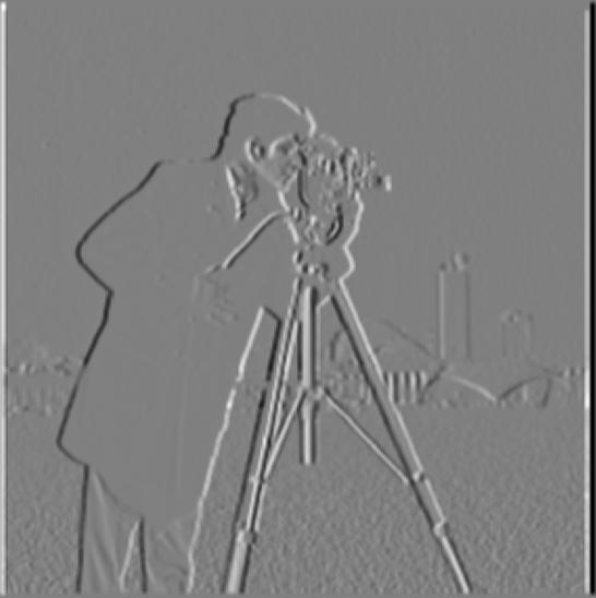
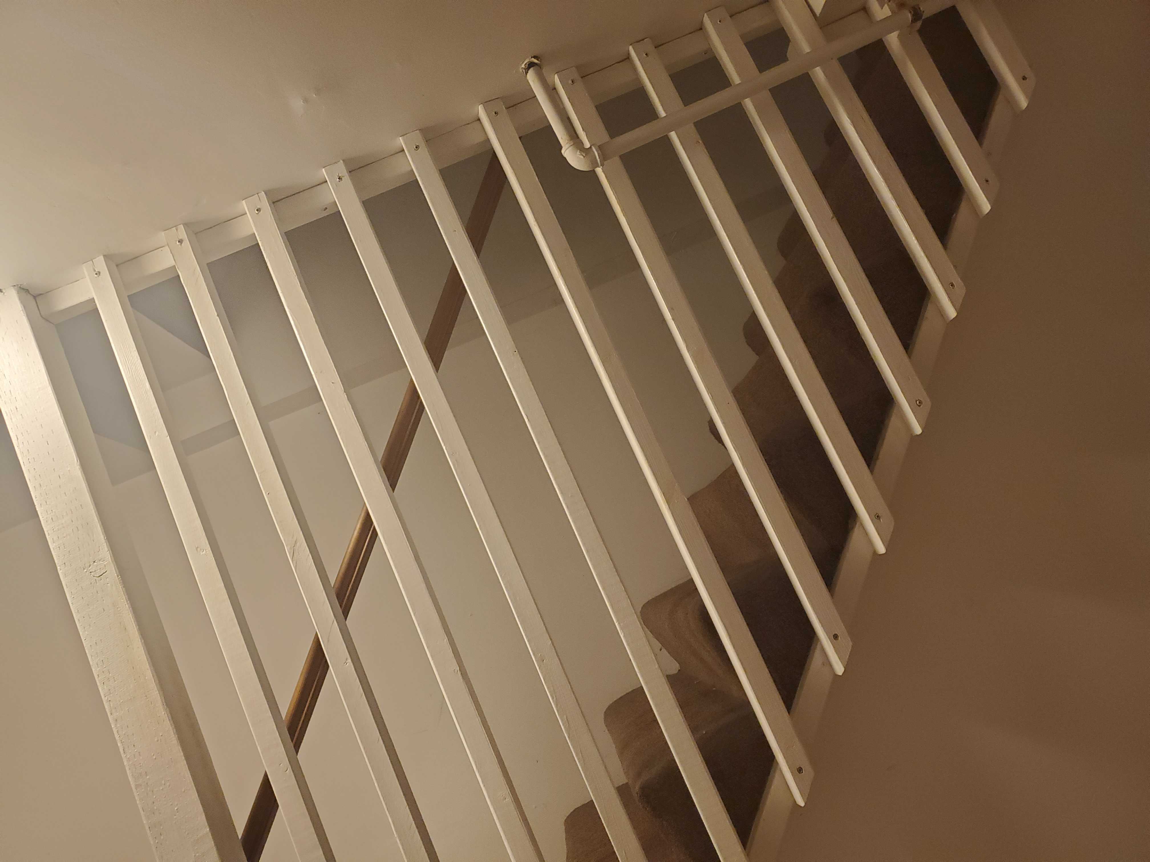
1.3 Image Straightening
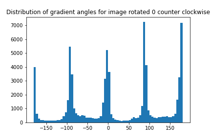
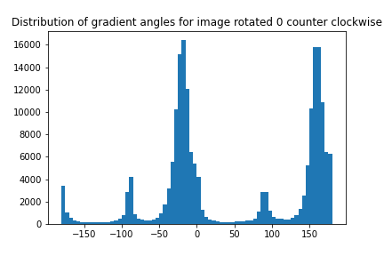
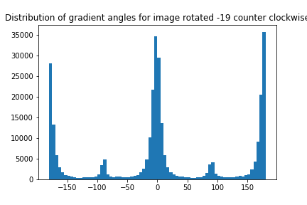
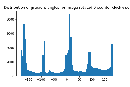
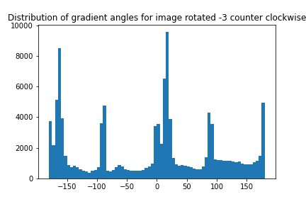
In this section, we attempt to automatically straighten images by rotating it to maximize the amount of "edges". We can compute the gradient angle of each pixel of an image by finding the tangent angle between the derivative of the image in the y direction and the derivative of the angle in the x direction.
The algorithm that produces the rotations below considers gradient angles that are close to 0, 90, 180, and 270 degrees as edges and filters gradient angles that have weak magnitude.
The rotated images on the right are additionally cropped to remove unnecessary borders that are produced from rotation algorithms.
rotation_angles = np.arange(-179, 180, 2)
num_edges = {}

img_path = 'stairs.jpg'
img = skio.imread(img_path, as_gray=True)

for angle in rotation_angles:
    # Rotate and crop image
    rotated = rotate(img, angle, mode='constant', reshape=True)
    crop_x = int(rotated.shape[0] * 0.3)
    crop_y = int(rotated.shape[1] * 0.3)
    rotated = rotated[crop_x:rotated.shape[0]-crop_x, crop_y:rotated.shape[1]-crop_y]

    # Convolve image with derivative of gaussian filter
    rotated_dx = convolve2d(rotated, gauss_dx)
    rotated_dy = convolve2d(rotated, gauss_dy)

    # Compute gradient angles/magnitudes
    grad_angles = np.arctan2(rotated_dy, rotated_dx)
    angle_mags = np.sqrt(rotated_dx**2 + rotated_dy**2)

    # Count proportion of edge pixels relative to total pixels
    total_edges = 0
    total_edges += ((grad_angles >= -0.001) & (grad_angles < 0.001))[angle_mags > 0.05].sum()
    total_edges += ((grad_angles >= np.pi/2-0.001) & (grad_angles < np.pi/2+0.001))[angle_mags > 0.05].sum()
    total_edges += ((grad_angles >= np.pi-0.001) & (grad_angles < np.pi+0.001))[angle_mags > 0.05].sum()
    total_edges += ((grad_angles >= 3*np.pi/2-0.001) & (grad_angles < 3*np.pi/2+0.001))[angle_mags > 0.05].sum()
    num_edges[angle] = total_edges / (grad_angles.shape[0] * grad_angles.shape[1])

#     print(angle, ': ', num_edges[angle])
#     sns.distplot((180/np.pi) * grad_angles[angle_mags > 0.05], kde=False)
#     plt.title(f'Distribution of Horizontal and Vertical Edges for Clockwise Rotation of {abs(angle)} degrees')
#     plt.show()
best_angle = max(num_edges, key=num_edges.get)
img = skio.imread(img_path, as_gray=True)
for angle in [0, best_angle]:
# Histogram of gradient angles (best angle)
rotated = rotate(img, angle, mode='constant', reshape=True)
crop_x = int(rotated.shape[0] * 0.3)
crop_y = int(rotated.shape[1] * 0.3)
rotated = rotated[crop_x:rotated.shape[0]-crop_x, crop_y:rotated.shape[1]-crop_y]
# Convolve image with derivative of gaussian filter
rotated_dx = convolve2d(rotated, gauss_dx)
rotated_dy = convolve2d(rotated, gauss_dy)
# Compute gradient angles/magnitudes
grad_angles = np.arctan2(rotated_dy, rotated_dx)
angle_mags = np.sqrt(rotated_dx**2 + rotated_dy**2)
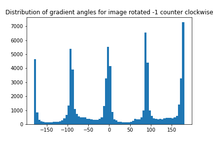
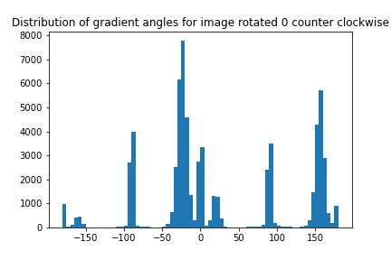
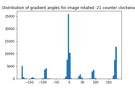
plt.hist((180/np.pi) * grad_angles[angle_mags > 0.05].flatten(), bins=np.arange(-180, 181, 5))
plt.title(f'Distribution of gradient angles for image rotated {angle} counter clockwise')
plt.savefig(f'{img_path}_hist_{angle}.png')
plt.xlabel('angle')
plt.ylabel('count')
plt.title('Distribution of gradient angles')
plt.clf()
img_path = 'stairs.jpg'
img = skio.imread(img_path, as_gray=False)
rotated_img = rotate(img, best_angle, reshape=True, mode='constant')
crop_x = int(rotated_img.shape[0] * 0.2)
crop_y = int(rotated_img.shape[1] * 0.2)
rotated_img = rotated_img[crop_x:rotated_img.shape[0]-crop_x, crop_y:rotated_img.shape[1]-crop_y]
skio.imshow(rotated_img)
skio.imsave(f'rotated_{img_path}', rotated_img)
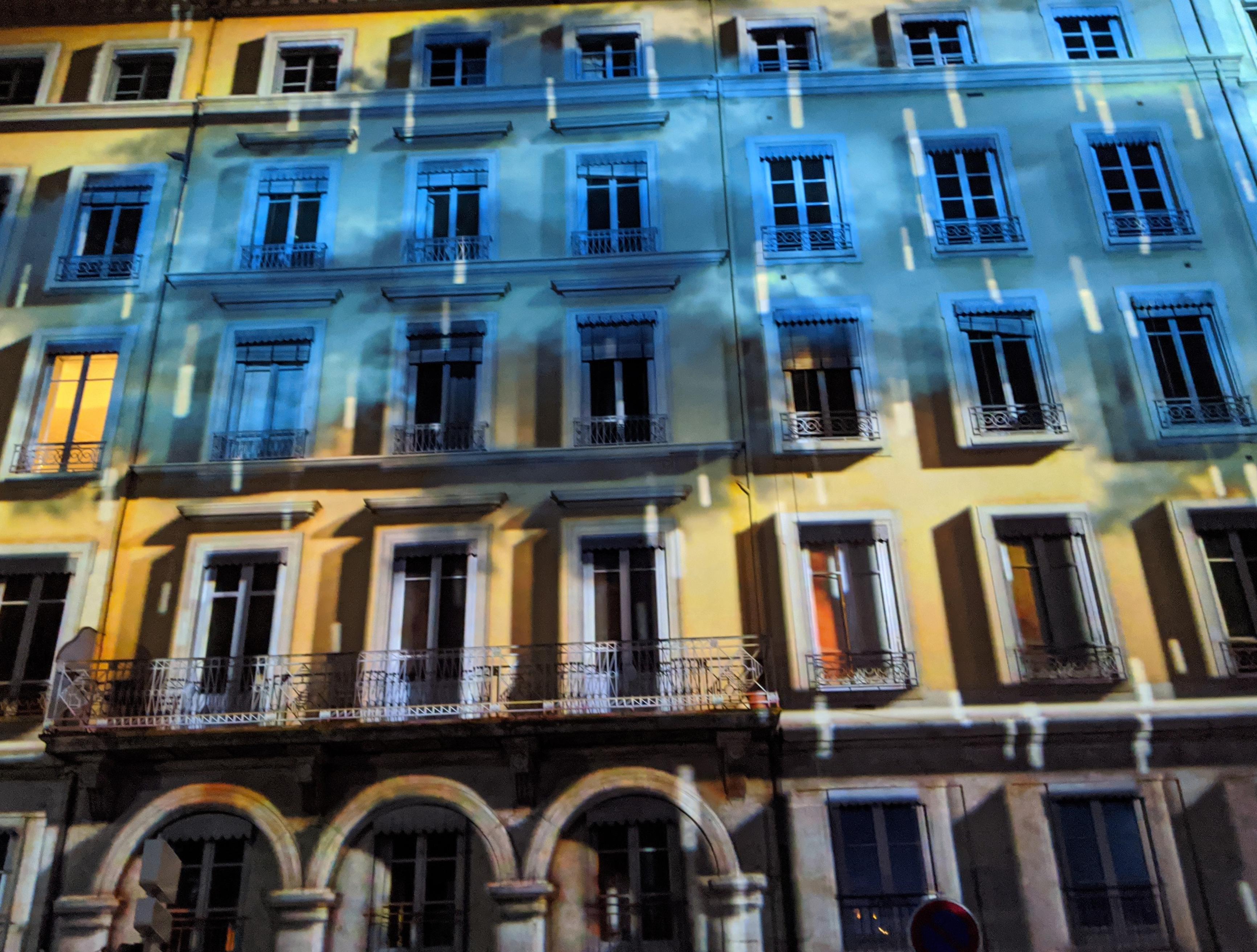
Facade
 |
 |
 |
 |
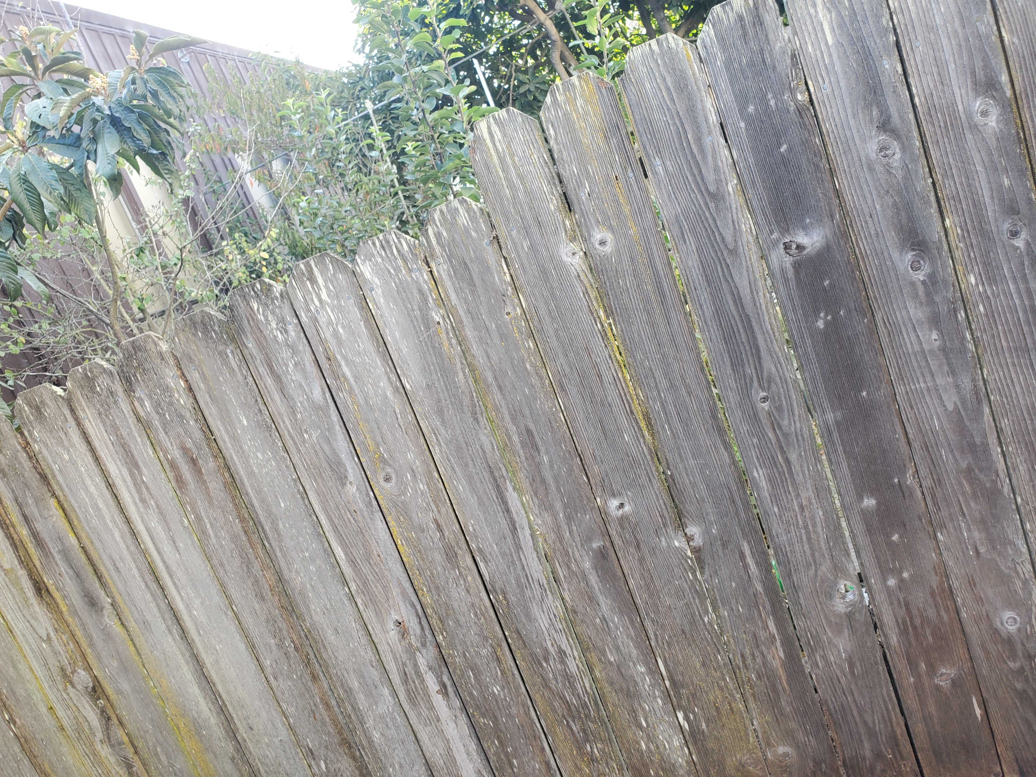
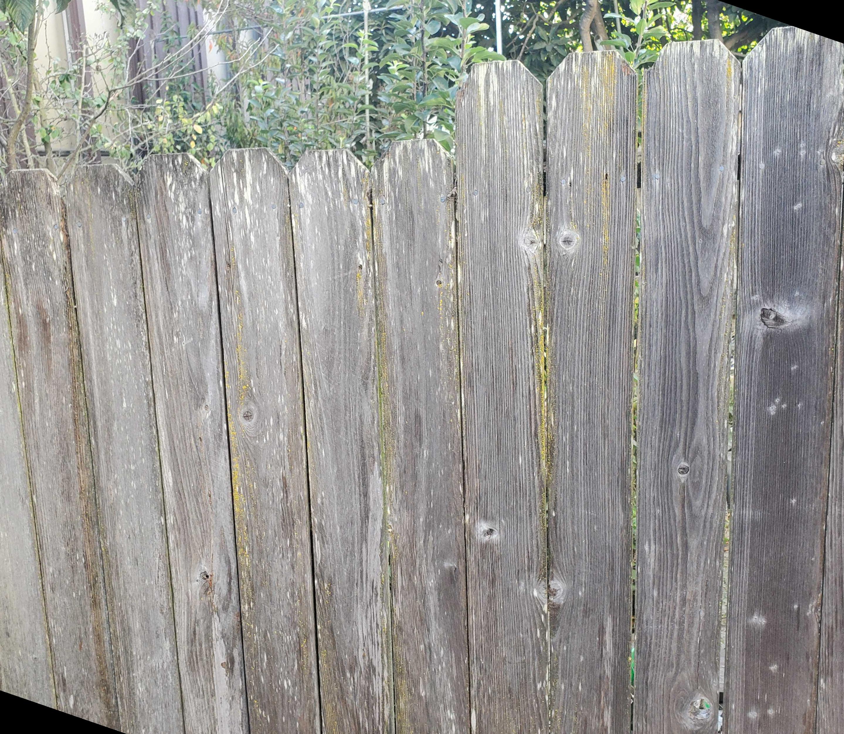
My Backyard Fence
 |
 |
 |
 |
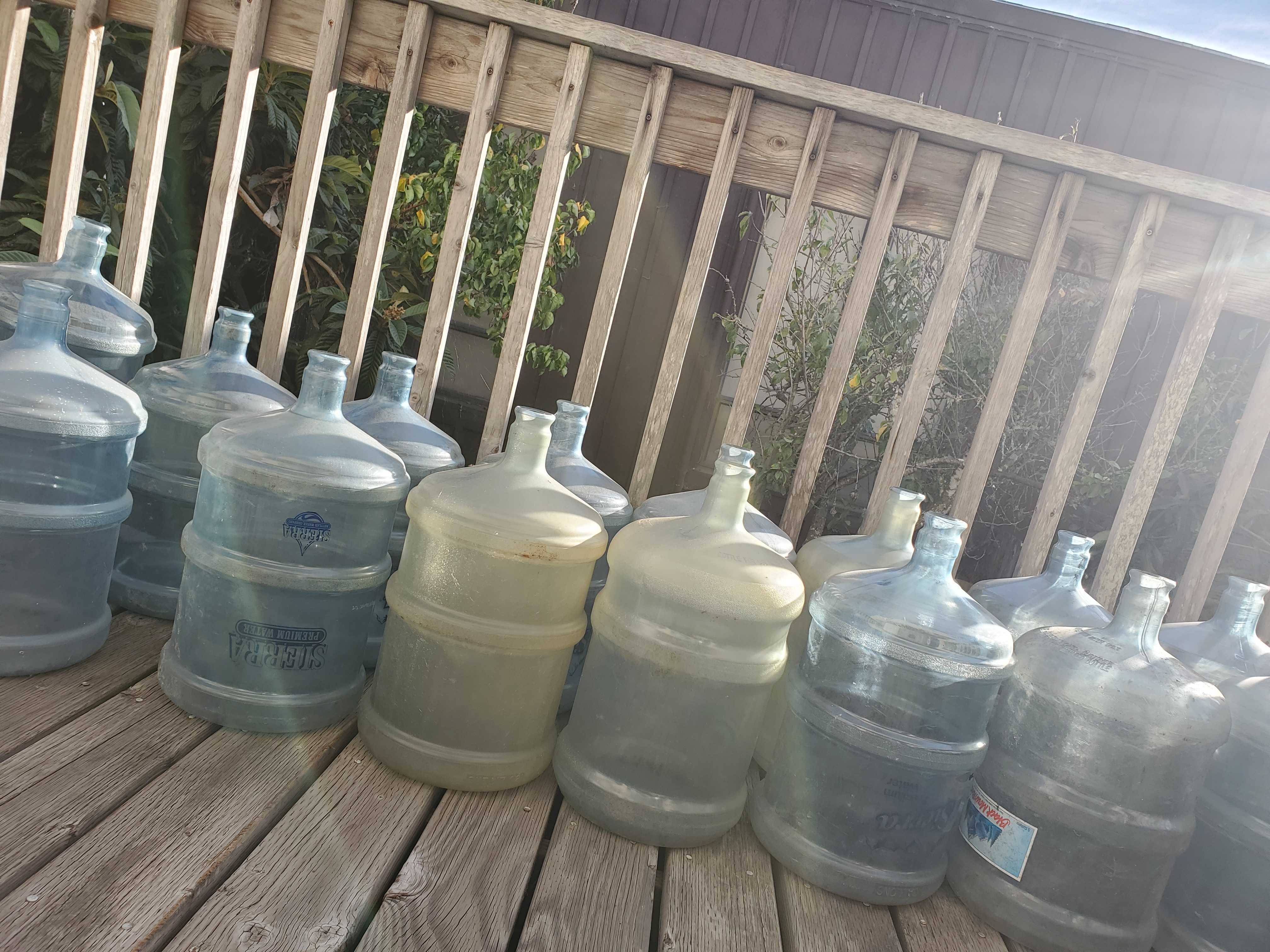
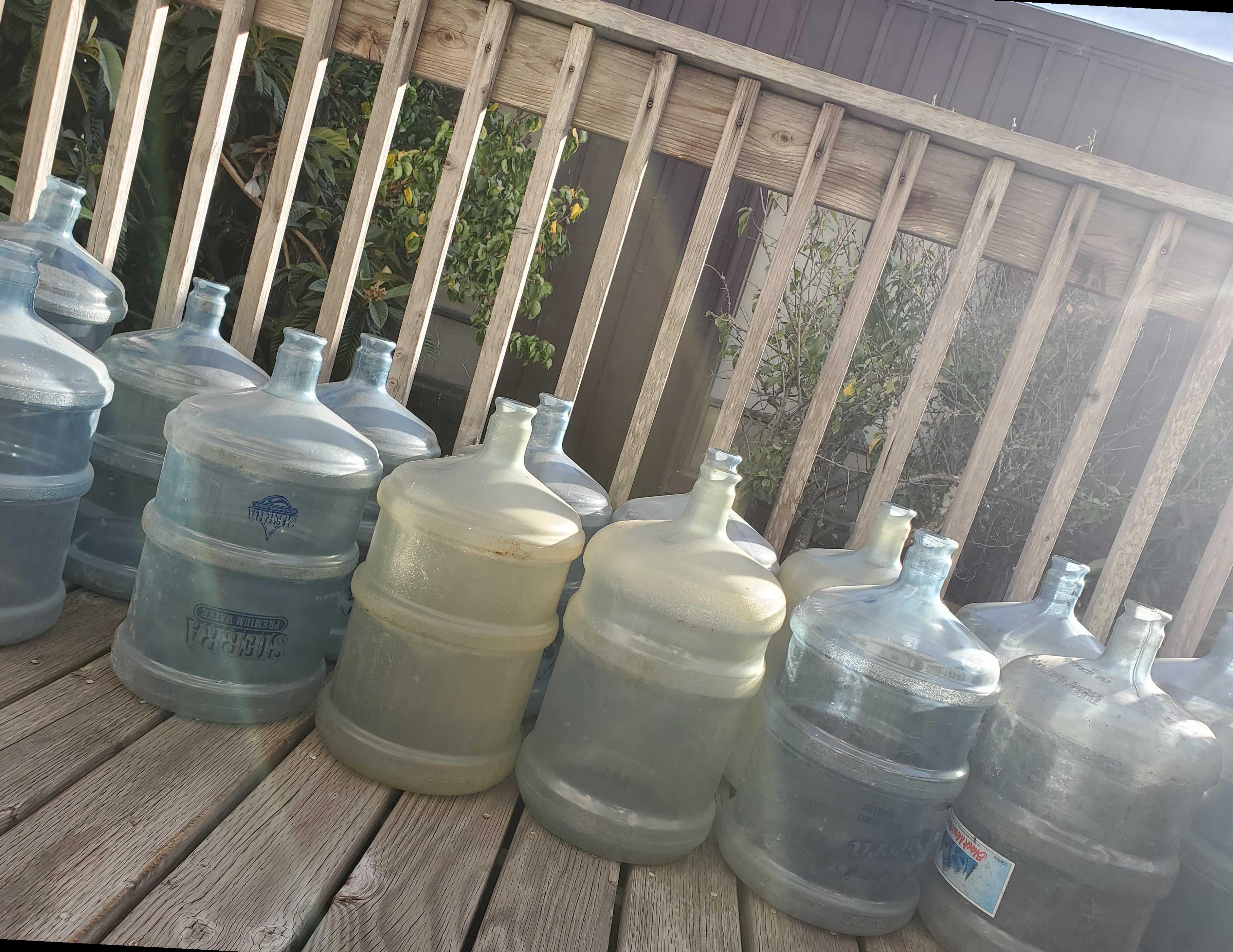
A bunch of watter bottles (also my backyard)
 |
 |
 |
 |
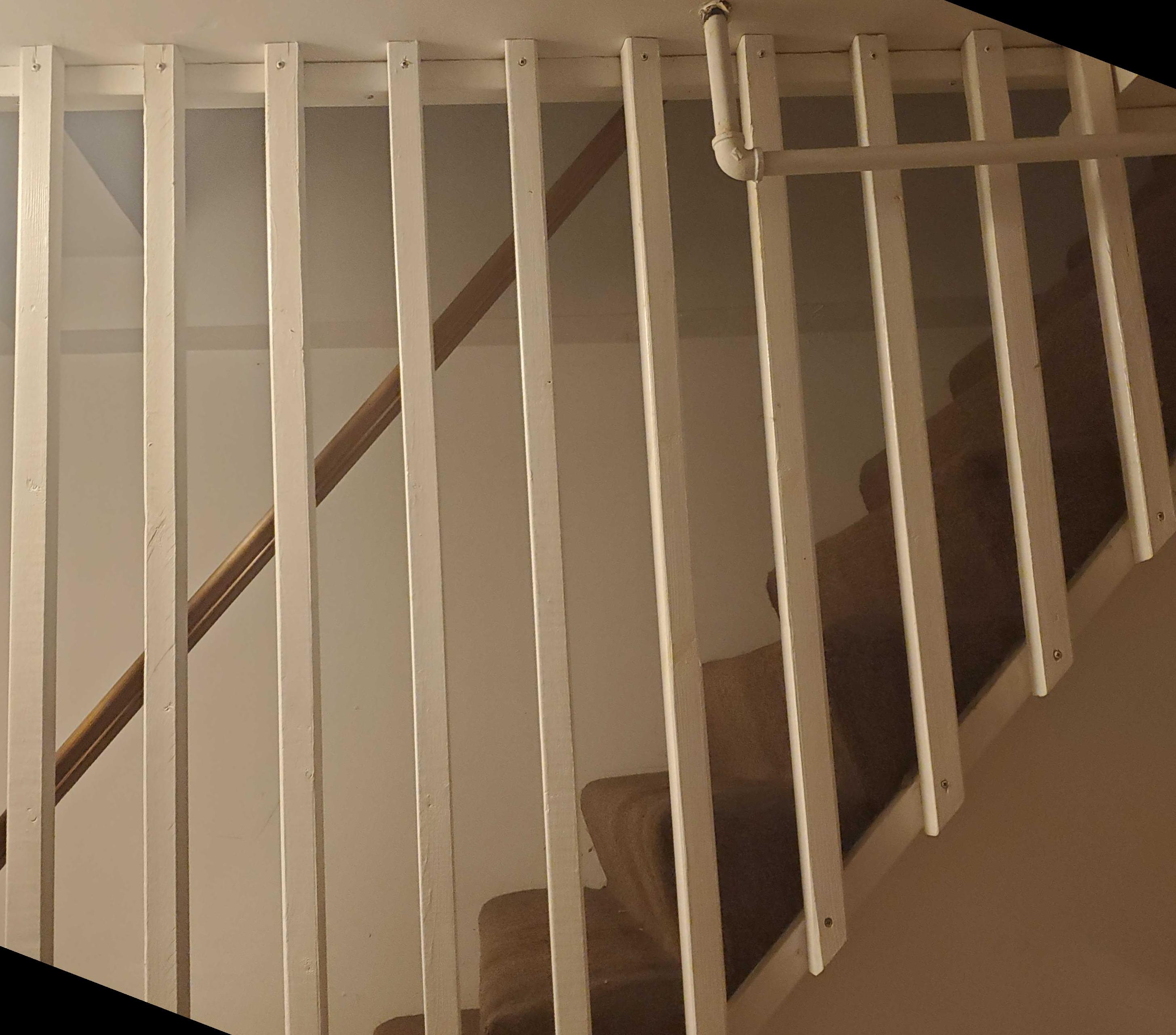
Stairs
 |
 |
 |
 |
Our rotation algorithm does an excellent job aside from the bottles images. We can see by inspection that a rotation of roughly 20 degrees counter clockwise would straighten the image, but my algorithm likely got confused by the strange pattern of the watter bottles and the wood markings which appear as edges.
Part 2: Fun with Frequencies!
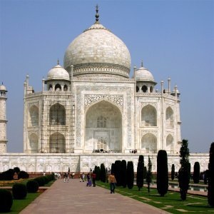
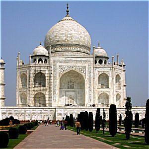
Part 2.1: Image "Sharpening"
In the next section, we apply an "unsharp" mask to an image to artificially make it appear sharper. We effectively achieve this by detecting the high frequency pixels in our image and adding only the high frequency pixels to our image.
taj = skio.imread('taj.jpg')
taj_r = taj[:, :, 0]
taj_g = taj[:, :, 1]
taj_b = taj[:, :, 2]
taj_smooth_r = convolve2d(taj_r, g_2d, mode='same')
taj_smooth_g = convolve2d(taj_g, g_2d, mode='same')
taj_smooth_b = convolve2d(taj_b, g_2d, mode='same')
alpha = 1
taj_sharp_r = taj_r + alpha * (taj_r - taj_smooth_r)
taj_sharp_g = taj_g + alpha * (taj_g - taj_smooth_g)
taj_sharp_b = taj_b + alpha * (taj_b - taj_smooth_b)
taj_sharp = np.dstack((taj_sharp_r, taj_sharp_g, taj_sharp_b))
taj_sharp = np.clip(taj_sharp, 0, 255)
skio.imsave('taj_sharp.jpg', taj_sharp)
Taj Mahal and Sharpened Taj Mahal
 |
 |
def sharpen(img_path, alpha):
    img = skio.imread(img_path)
    skio.imshow(img)
    img_r = img[:, :, 0]
    img_g = img[:, :, 1]
    img_b = img[:, :, 2]
    img_smooth_r = convolve2d(img_r, g_2d, mode='same')
    img_smooth_g = convolve2d(img_g, g_2d, mode='same')
    img_smooth_b = convolve2d(img_b, g_2d, mode='same')
    img_sharp_r = img_r + alpha * (img_r - img_smooth_r)
    img_sharp_g = img_g + alpha * (img_g - img_smooth_g)
    img_sharp_b = img_b + alpha * (img_b - img_smooth_b)
    img_sharp = np.dstack((img_sharp_r, img_sharp_g, img_sharp_b))
    img_sharp = np.clip(img_sharp, 0, 255)
    skio.imsave(f'{img_path}_sharp.jpg', img_sharp)
    skio.imshow(img_sharp/255)
We can also make the sharpening process more efficient by rearranging the operations of our convolution:
$f + \alpha(f - f\star g) = f\star ((1+\alpha)e - \alpha g)$
Where $\star$ denotes a convolution, f is our original image, g is the smoothed image, and e is the unit impulse.
Below are a few more examples of images before and after they've been sharpened!
unit_impulse = np.zeros((g_2d.shape[0], g_2d.shape[1]))
unit_impulse[2:4, 2:4] = 1
def sharpen_efficient(img_path, alpha):
    img = skio.imread(img_path)
    skio.imshow(img)
    img_r = img[:, :, 0]
    img_g = img[:, :, 1]
    img_b = img[:, :, 2]
    ag = g_2d * alpha
    conv_exp = (1+alpha)*unit_impulse - ag
    img_sharp_r = convolve2d(img_r, conv_exp, mode='same')
    img_sharp_g = convolve2d(img_g, conv_exp, mode='same')
    img_sharp_b = convolve2d(img_b, conv_exp, mode='same')
    img_sharp = np.dstack((img_sharp_r, img_sharp_g, img_sharp_b))
    img_sharp = np.clip(img_sharp, 0, 255)
    skio.imsave(f'{img_path}_sharp', img_sharp)
    skio.imshow(img_sharp/255)
# sharpen('cars.jpg', 10)
# sharpen('forest.jpg', 5)
 |
 |
 |
 |
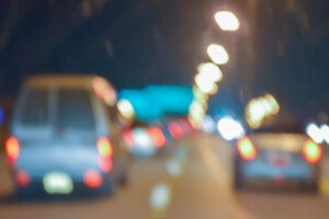
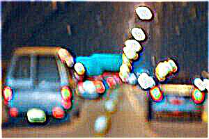
Next, we attempt to re-sharpen an already sharp image by blurring it first...
# img = skio.imread('road.jpg')
# skio.imshow(img)
# img_r, img_g, img_b = img[:, :, 0], img[:, :, 1], img[:, :, 2]
# img_blurry = np.dstack((convolve2d(img_r, g_2d),
#                          convolve2d(img_g, g_2d),
#                          convolve2d(img_b, g_2d)))
# skio.imshow(img/255)
# skio.imsave('road_blurry.jpg', img_blurry)
# sharpen('road_blurry.jpg', 5)
Original (Left), Blurred (Middle), Re-sharpened (Right)
 |
 |
 |
We see that the resharpened image is not nearly as beautiful as the original (the sharper pixels are overemphasized and look artificial)
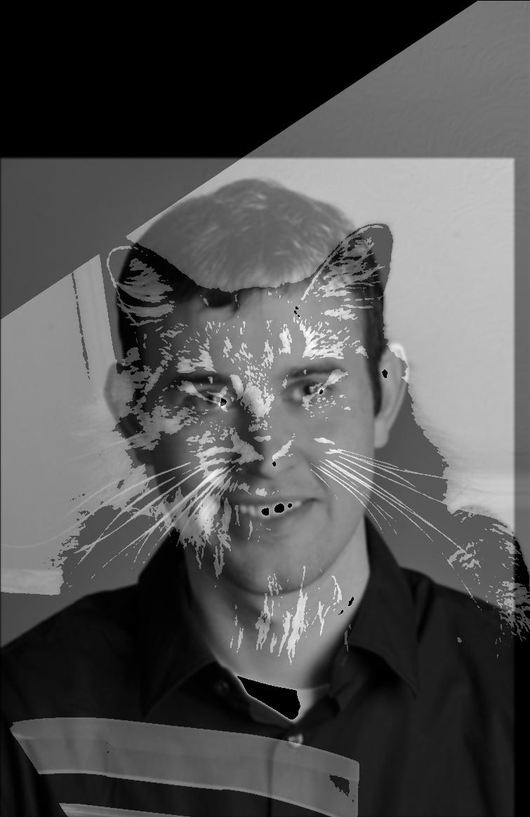
Part 2.2 Hybrid Images
We can create hybrid images that appear differently depending on how close or far away you view the image by modifying each image to either only have low or high frequencies and combining the two images. The low frequency image should appear at further distances, while the high frequency image should appear at closer distances.
import align_image_code
from align_image_code import align_images
import matplotlib
%matplotlib inline
# First load images
matplotlib.use('TkAgg')
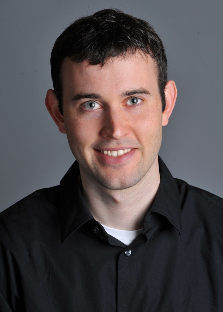
im1 = plt.imread('./DerekPicture.jpg')/255.
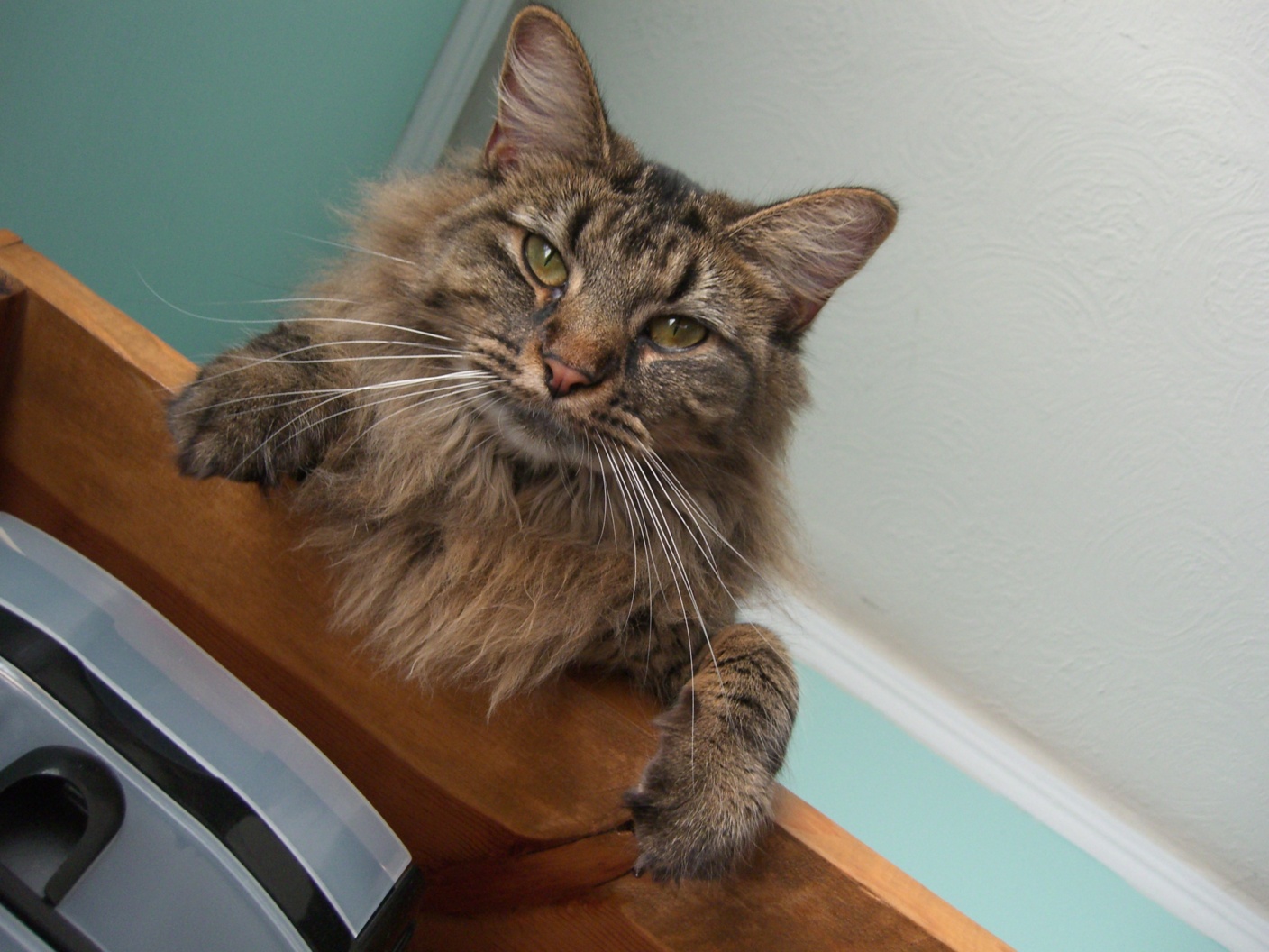
im2 = plt.imread('./nutmeg.jpg')/255
# Next align images (this code is provided, but may be improved)
im2_aligned, im1_aligned = align_images(im2, im1)
## Derek should be low pass (gaussian filter), Nutmeg should be highpass (impulse - gaussian)

matplotlib.use('module://ipykernel.pylab.backend_inline')
plt.subplot(1, 2, 1)
plt.imshow(im2_aligned);

plt.subplot(1, 2, 2)
plt.imshow(im1_aligned);
sigma1 = 0.8
sigma2 = 3
im2_aligned = sc.rgb2gray(im2_aligned)
im1_aligned = sc.rgb2gray(im1_aligned)
im1_blurred = convolve2d(im1_aligned, g_2d, mode='same')
im1_blurred = (im1_blurred < sigma1) * im1_blurred
skio.imshow(im1_blurred, cmap='gray')
alpha = 1
im2_sharpened = convolve2d(im2_aligned, (1+alpha)*unit_impulse - alpha*g_2d, mode='same')
im2_sharpened = (im2_sharpened > sigma2) * im2_sharpened
skio.imshow(im2_sharpened)
combined_image = (im1_blurred + im2_sharpened*0.1)
plt.imshow(combined_image, cmap='gray')
skio.imsave('combined.jpg', combined_image);
def merge_images(img1, img2, sigma1, sigma2):

    #img1 = low frequency
    #img2 = high frequency
    # First load images


    %matplotlib inline
    matplotlib.use('TkAgg')

    im1 = plt.imread(img1)/255.
    im2 = plt.imread(img2)/255
    im2_aligned, im1_aligned = align_images(im2, im1)

    matplotlib.use('module://ipykernel.pylab.backend_inline')
#     plt.subplot(1, 2, 1)
#     plt.imshow(im2_aligned);

#     plt.subplot(1, 2, 2)
#     plt.imshow(im1_aligned);

    # convert to grayscale
    im2_aligned = sc.rgb2gray(im2_aligned)
    im1_aligned = sc.rgb2gray(im1_aligned)

    # Apply gaussian blur filter to img 1
    im1_blurred = convolve2d(im1_aligned, g_2d, mode='same')
    im1_blurred = (im1_blurred < sigma1) * im1_blurred

    # Sharpen img 2 by convovling with laplacian of gaussian
    alpha = 1
    im2_sharpened = convolve2d(im2_aligned, (1+alpha)*unit_impulse - alpha*g_2d, mode='same')
    im2_sharpened = (im2_sharpened > sigma2) * im2_sharpened

    # Weighted sum of img1 and 0.1*img2
    combined_image = (im1_blurred + im2_sharpened*0.1)
    skio.imsave(f'{img1}_{img2}', combined_image);
Derek (Low), Nutmeg (High), and Combined Derek & Nutmeg (terrifying)
 |
 |
 |
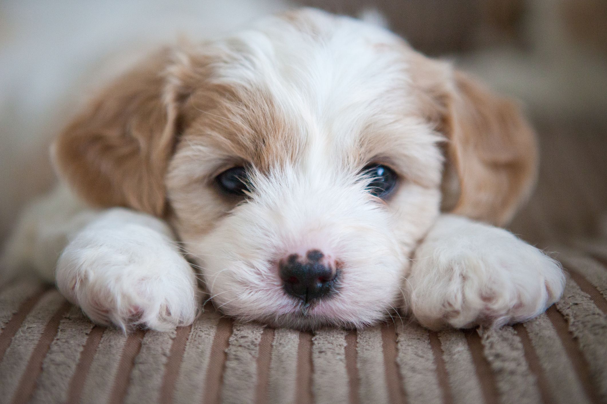
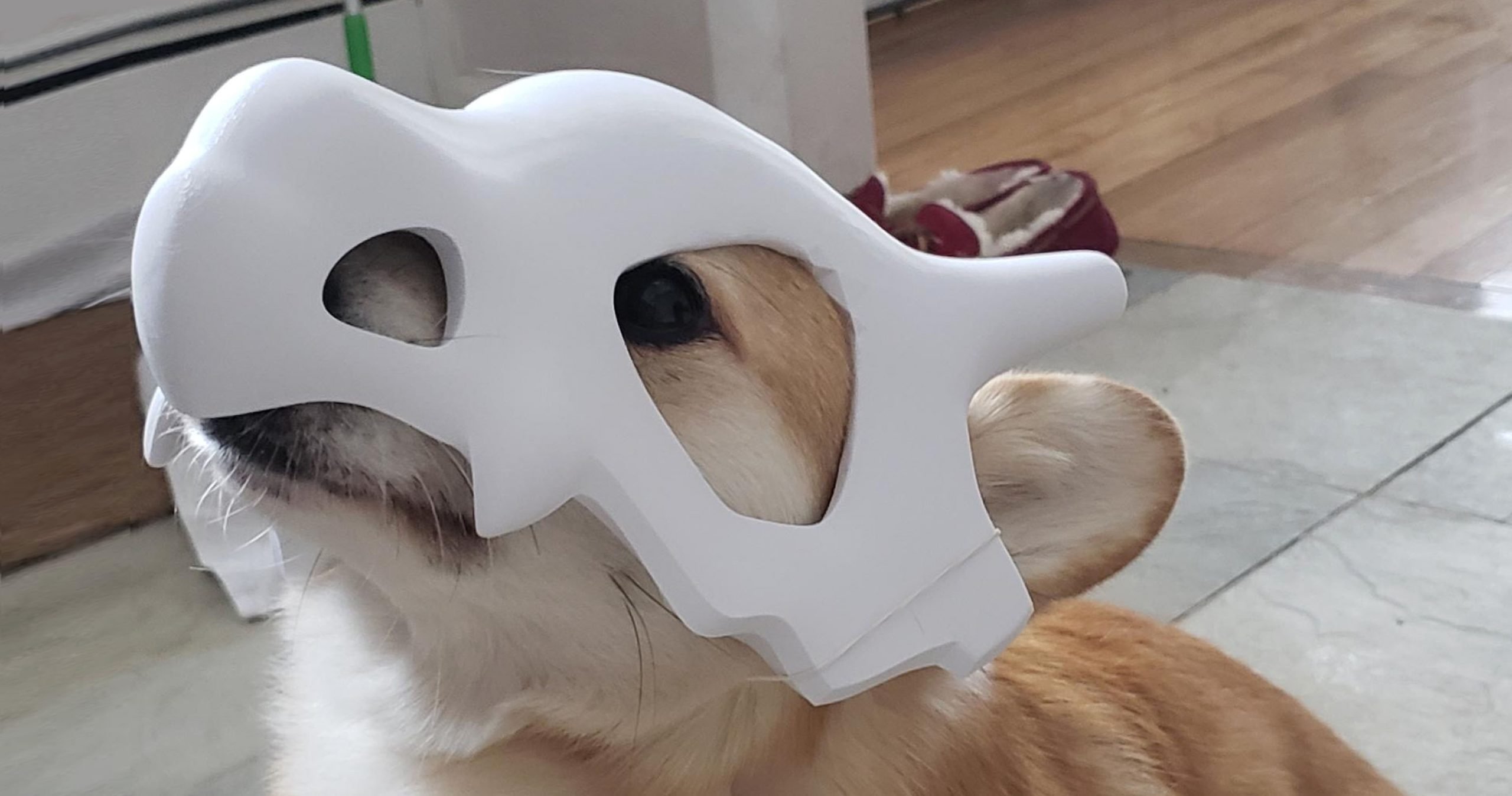
merge_images('cubone.jpg', 'puppy.jpg', 0.8, 4)
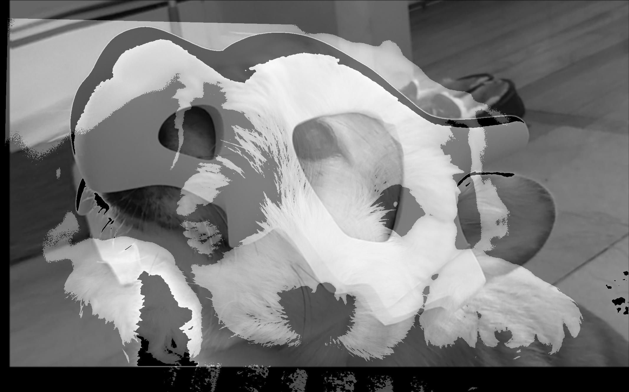
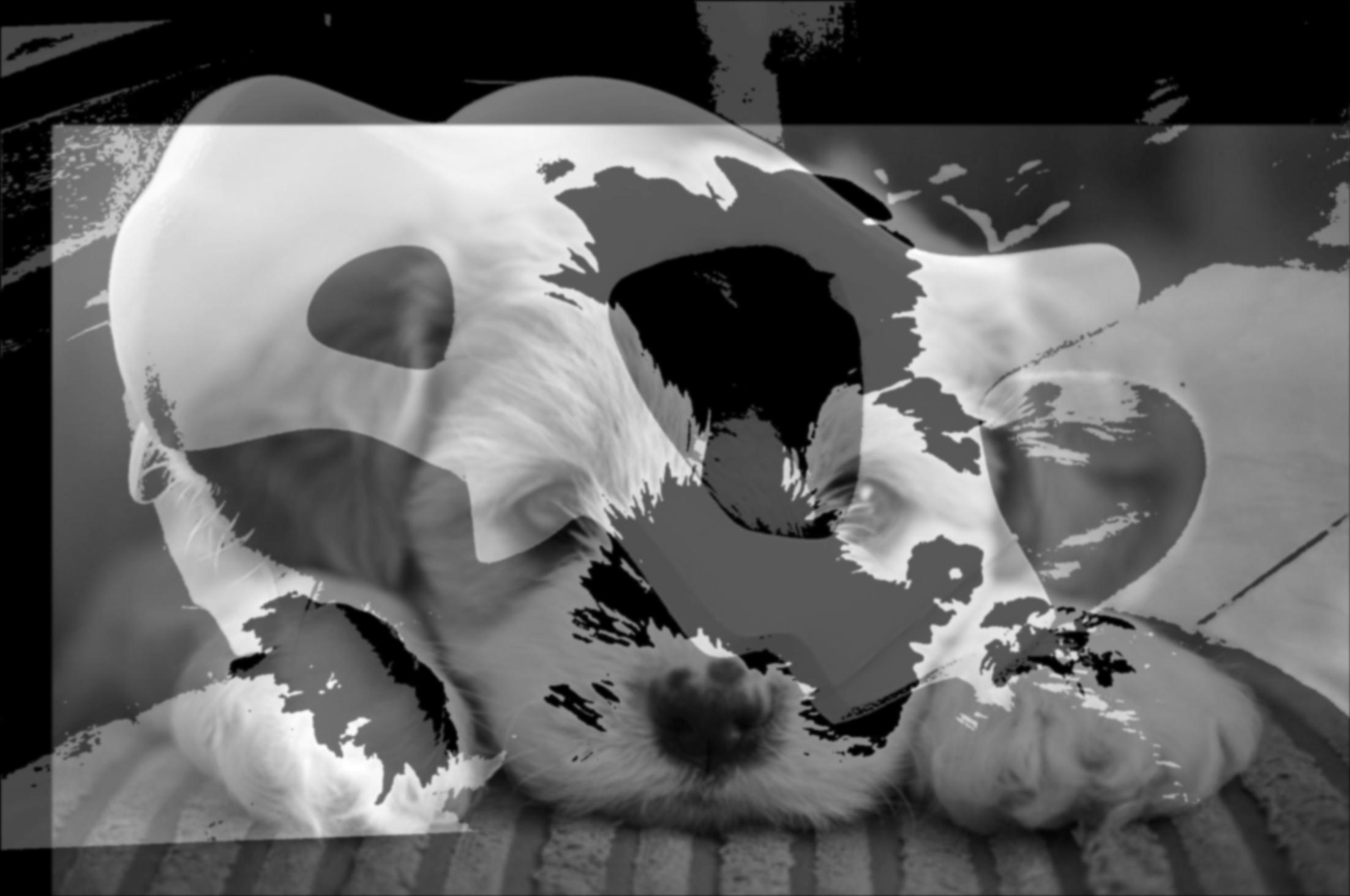
Puppy (low), Cubone Puppy (high), Combined (awww)
 |
 |
 |
from align_image_code import align_images
import matplotlib
%matplotlib inline
matplotlib.use('TkAgg')

im1 = plt.imread('cubone.jpg')/255.
im2 = plt.imread('puppy.jpg')/255
im2_aligned, im1_aligned = align_images(im2, im1)

matplotlib.use('module://ipykernel.pylab.backend_inline')
plt.subplot(1, 2, 1)
plt.imshow(im2_aligned);

plt.subplot(1, 2, 2)
plt.imshow(im1_aligned);

# convert to grayscale
im2_aligned = sc.rgb2gray(im2_aligned)
im1_aligned = sc.rgb2gray(im1_aligned)
Below, we illustrate the process through frequency analysis by showing the log magnitude of the Fourier transform between the Puppy and Cubone images
Log FFT Transform of Original Images
plt.subplot(1, 2, 1)
plt.title('Log Fourier (puppy)')
plt.imshow(np.log(np.abs(np.fft.fftshift(np.fft.fft2(im2_aligned)))))

plt.subplot(1, 2, 2)
plt.title('Log Fourier Transform (cubone)')
plt.imshow(np.log(np.abs(np.fft.fftshift(np.fft.fft2(im1_aligned)))));

Log FFT Transform of Filtered Images
# Apply gaussian blur filter to img 1
im1_blurred = convolve2d(im1_aligned, g_2d, mode='same')
im1_blurred = (im1_blurred < sigma1) * im1_blurred

# Sharpen img 2 by convovling with laplacian of gaussian
alpha = 1
im2_sharpened = convolve2d(im2_aligned, (1+alpha)*unit_impulse - alpha*g_2d, mode='same')
im2_sharpened = (im2_sharpened > sigma2) * im2_sharpened

plt.subplot(1, 2, 1)
plt.title('Log Fourier (puppy blurred)')
plt.imshow(np.log(np.abs(np.fft.fftshift(np.fft.fft2(im1_blurred)))));

plt.subplot(1, 2, 2)
plt.title('Log Fourier (cubone sharpened)')
plt.imshow(np.log(np.abs(np.fft.fftshift(np.fft.fft2(im2_sharpened)))))

Log FFT Transform on Hybrid Image
combined = skio.imread('puppy.jpg_cubone.jpg', as_gray=True)
plt.title('Log Fourier (Combined Image))')
plt.imshow(np.log(np.abs(np.fft.fftshift(np.fft.fft2(combined)))))

# %matplotlib inline
# matplotlib.use('TkAgg')
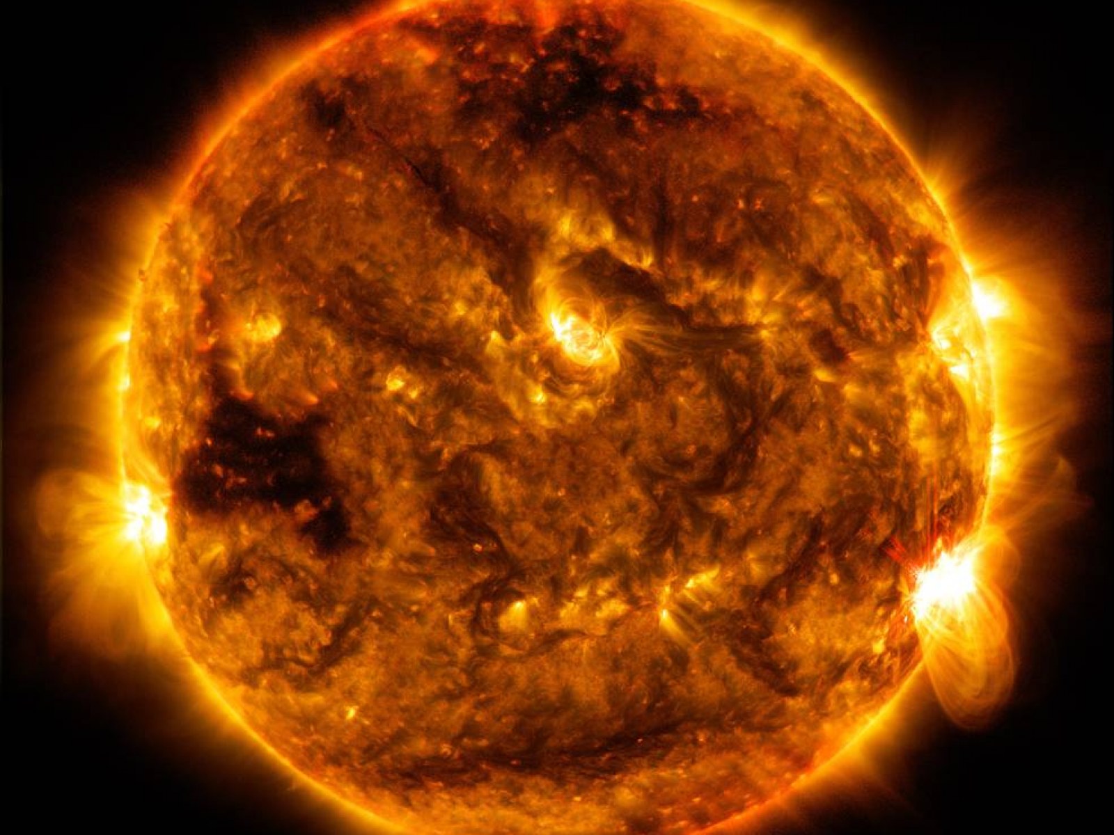
# merge_images('sun.jpg', 'saturn.jpg', 0.7, 4)
# skio.imshow(skio.imread('sun.jpg_saturn.jpg'))
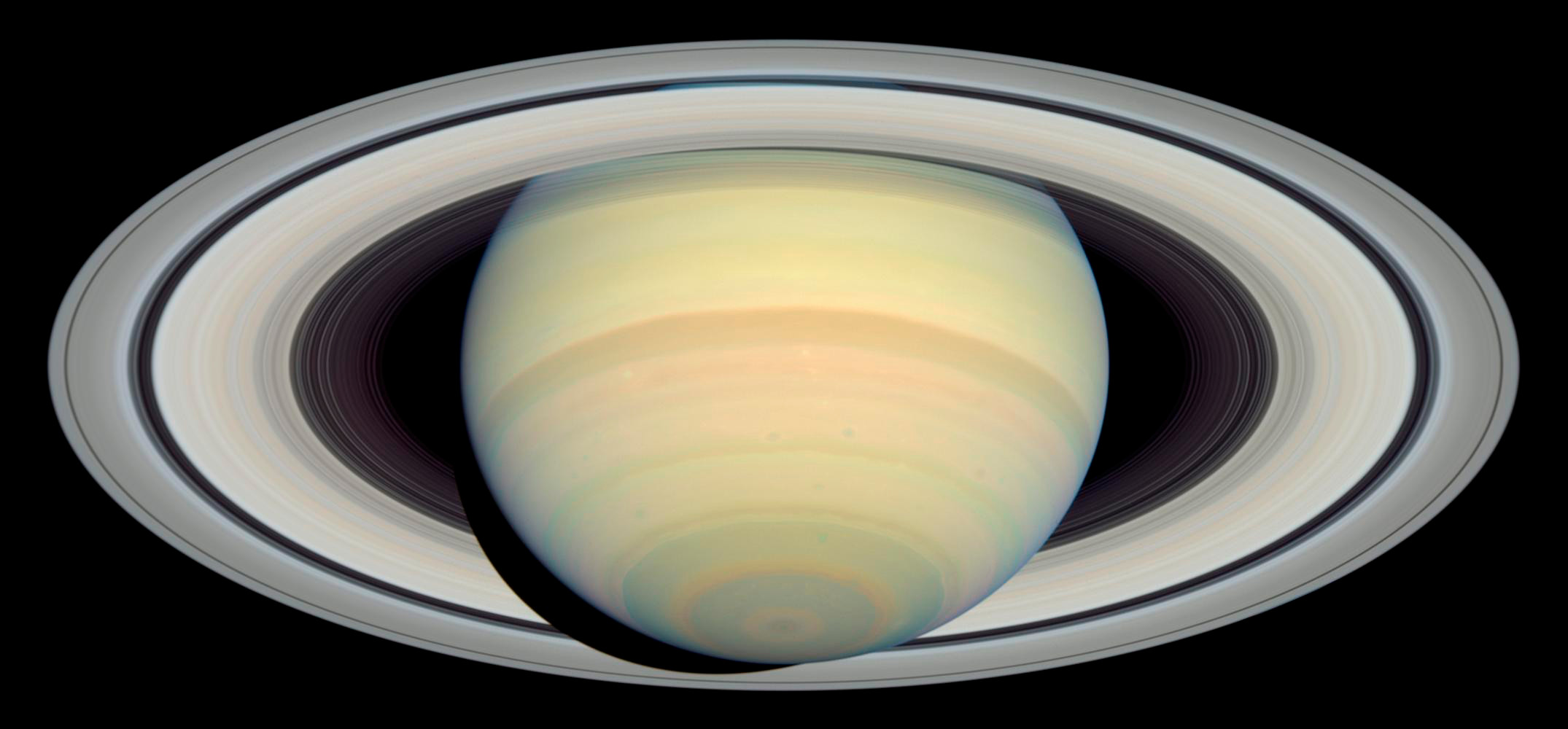
Saturn (Low), Sun (High), Sun of Saturn (???)
 |
 |
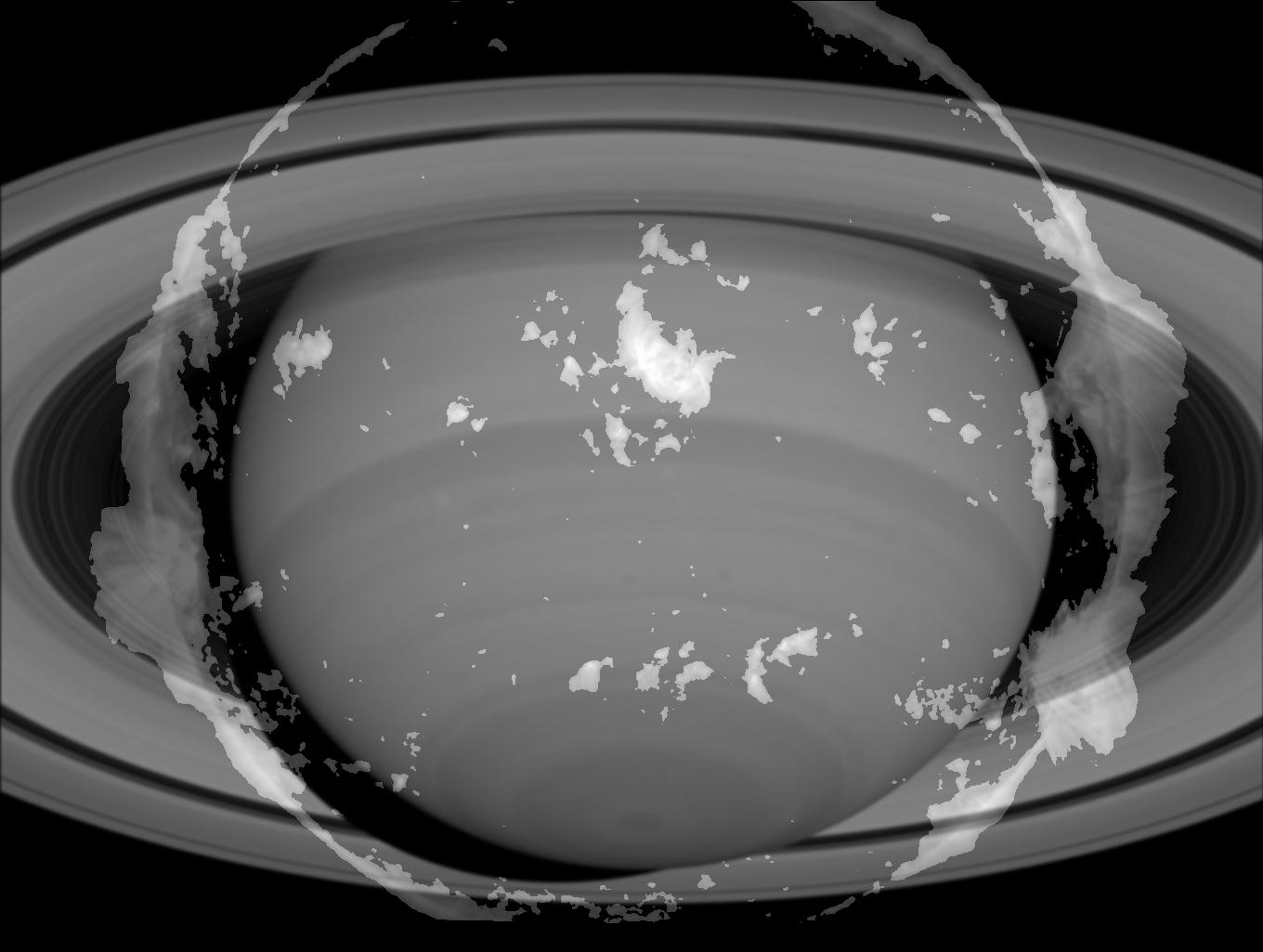 |
Our combined Sun and Saturn image is not particularly successful because it looks roughly the same from close and far distances. This is likely due to the fact that the images are not that different in the first place (especially when grayscaled) and one happens to be much brighter than the other.
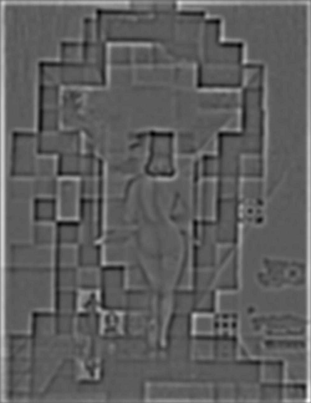
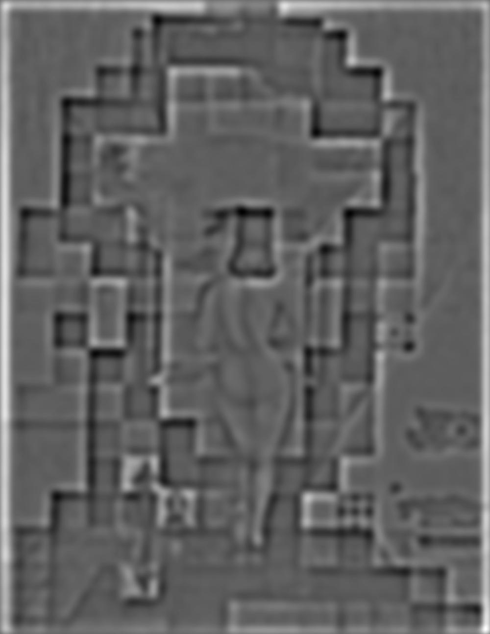
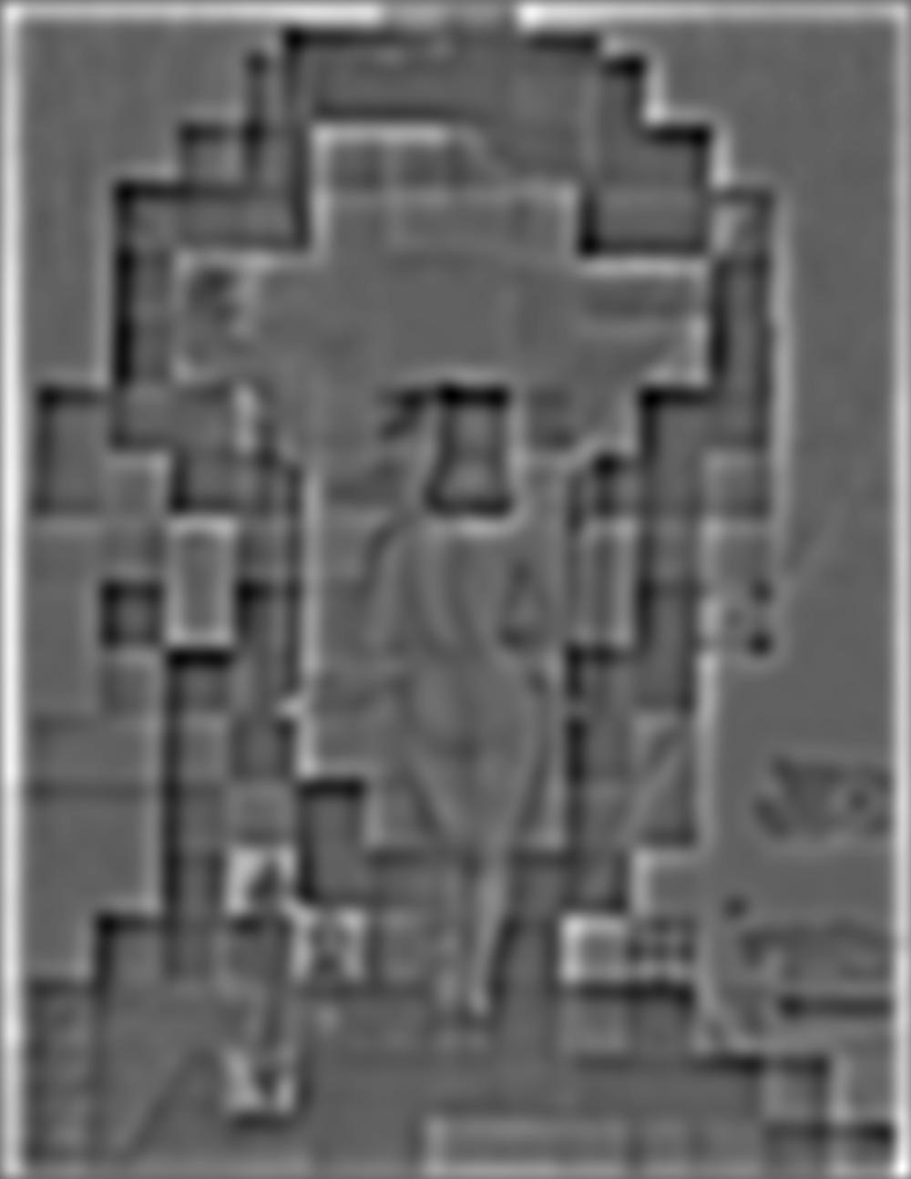
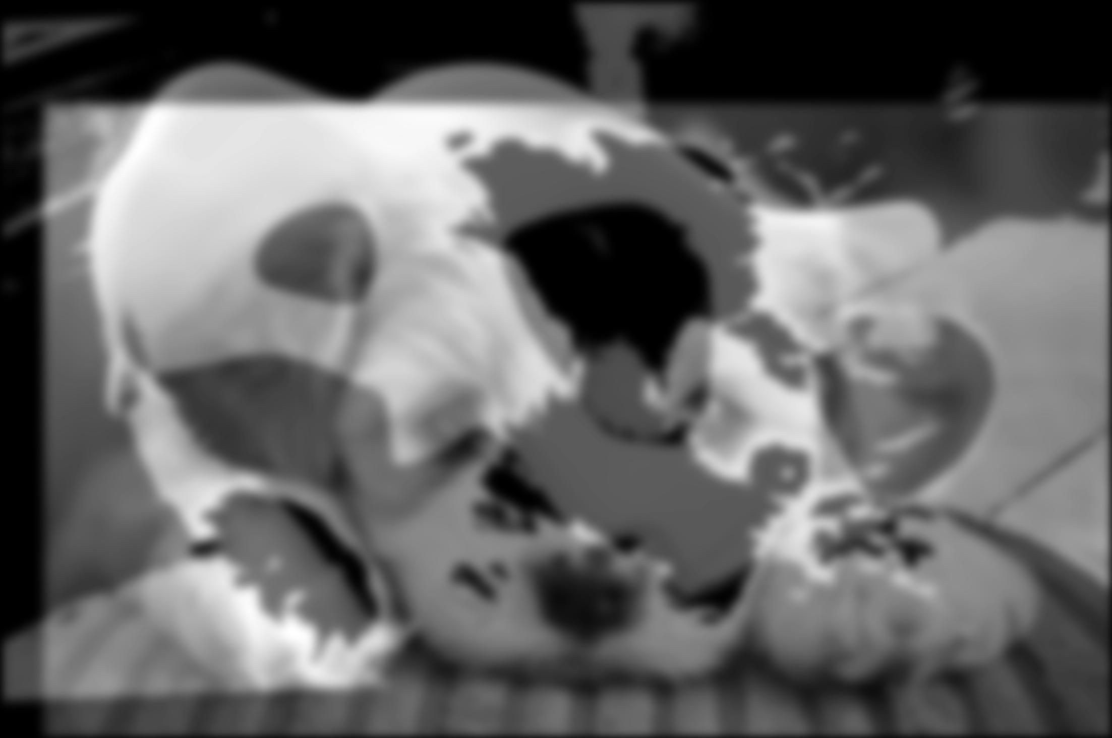
Part 2.3 Gaussian and Laplacian Stacks
# lincoln = skio.imread('lincoln.jpg')
# skio.imshow(lincoln)
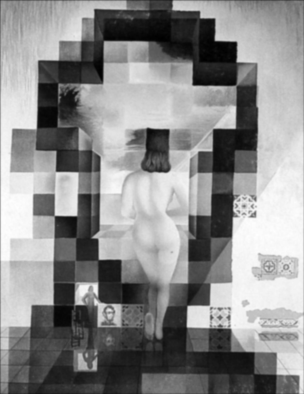
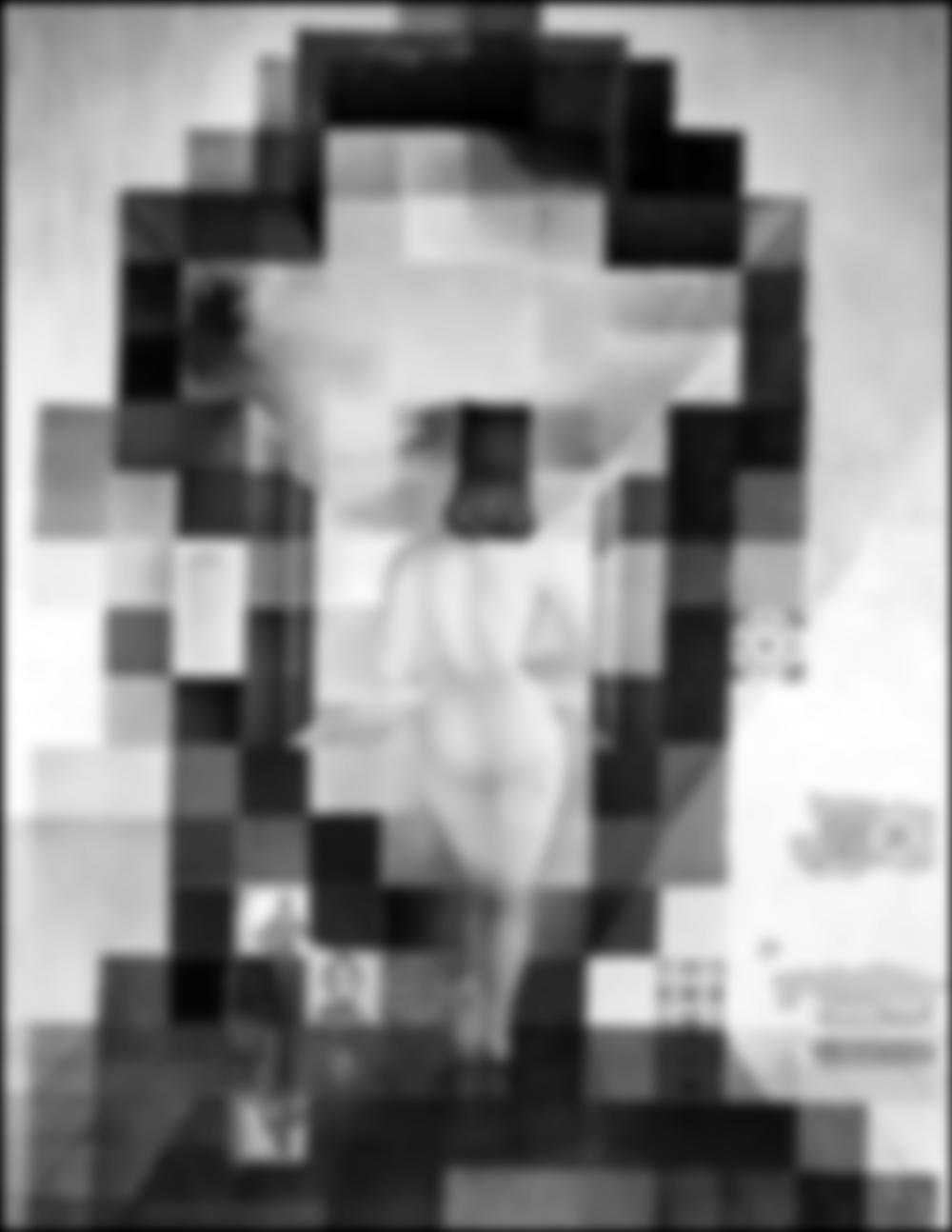
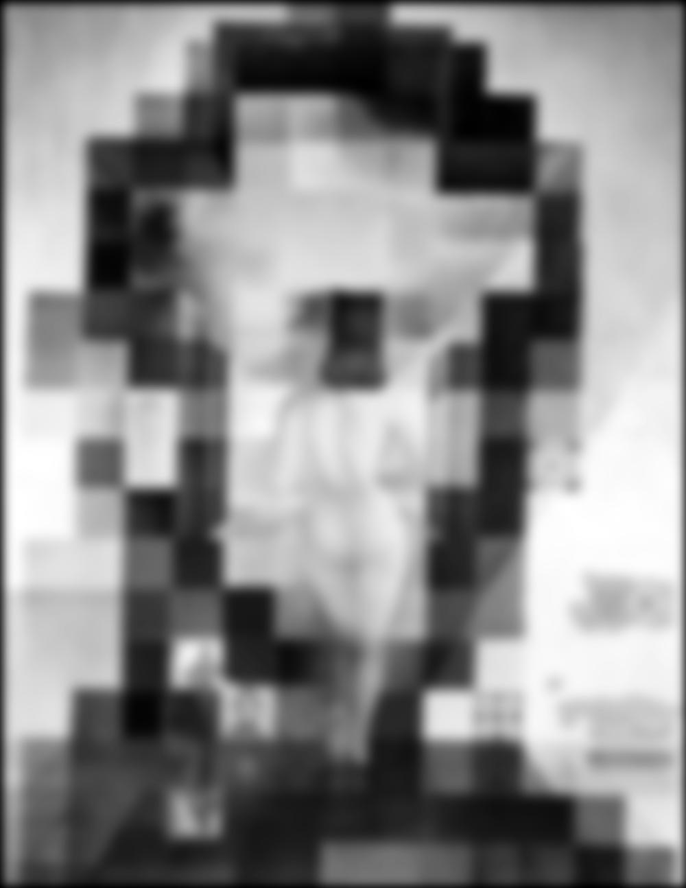
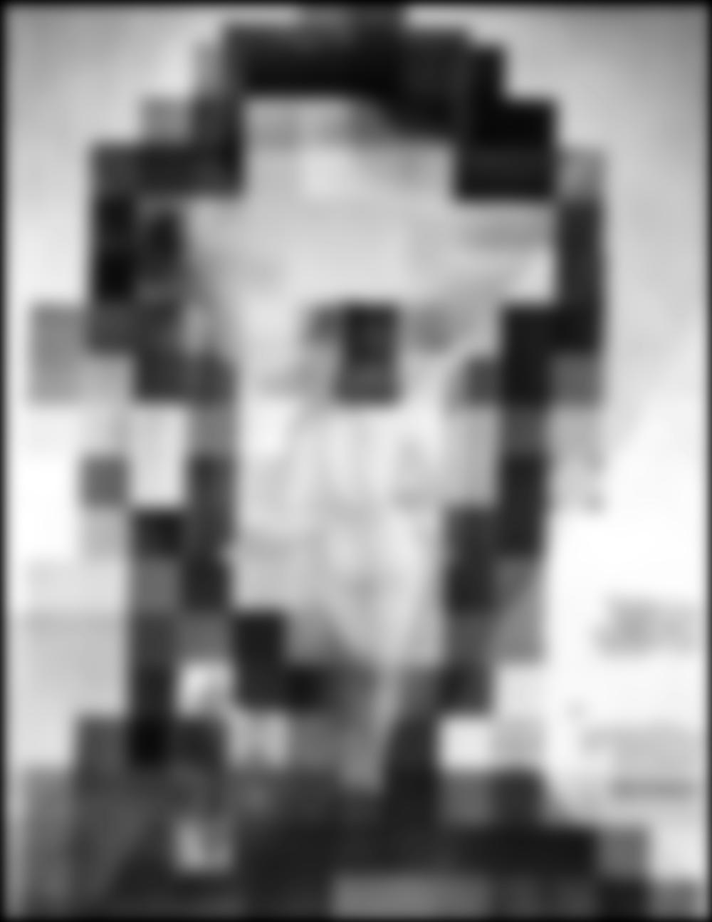
To create a gaussian stack (identical to a gaussian pyramid without downsampling), we convolute our original image by a multiplcatively increasing sigma (standard deviation parameter of gaussian filter) at each level, where the input at each layer is the result of prior layer. Here, we begin with a gaussian kernel where $\sigma=2$ and $\sigma$ is doubled at each layer.
Gaussian Stack of Lincoln in Dalivision
gaussian_stack = []
blurred = sc.rgb2gray(lincoln)
for i in range(1, 7):
    g_new = cv2.getGaussianKernel(ksize=20, sigma=2**i)
    g_new2d = g_new @ g_new.T
    blurred = convolve2d(blurred, g_new2d, mode='same')
    gaussian_stack.append(blurred)
    plt.imsave(f'lincoln_{i}.jpg', blurred, cmap='gray')
 |
 |
 |
 |
 |
 |
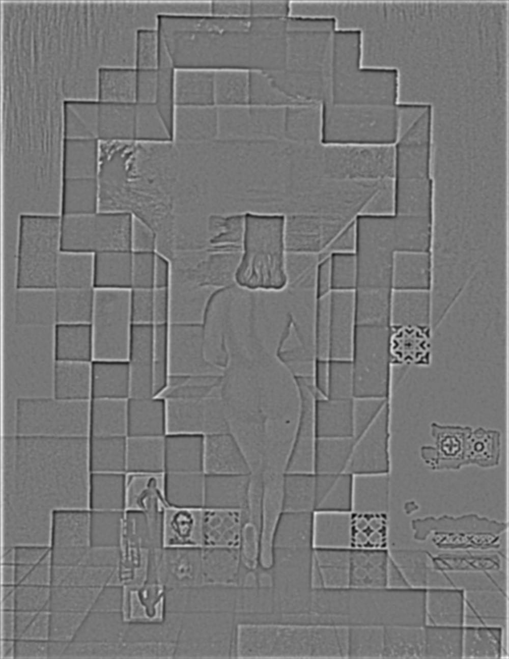
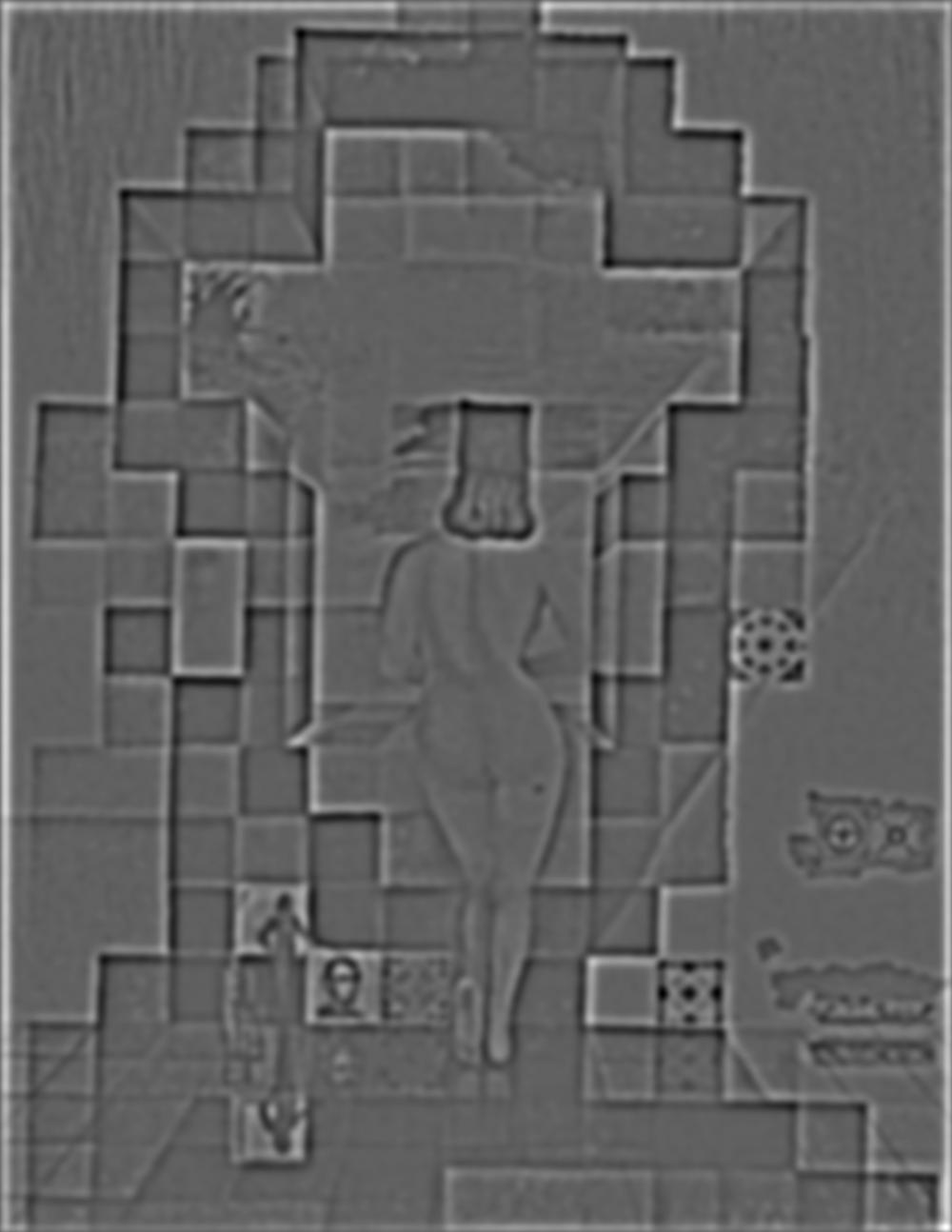
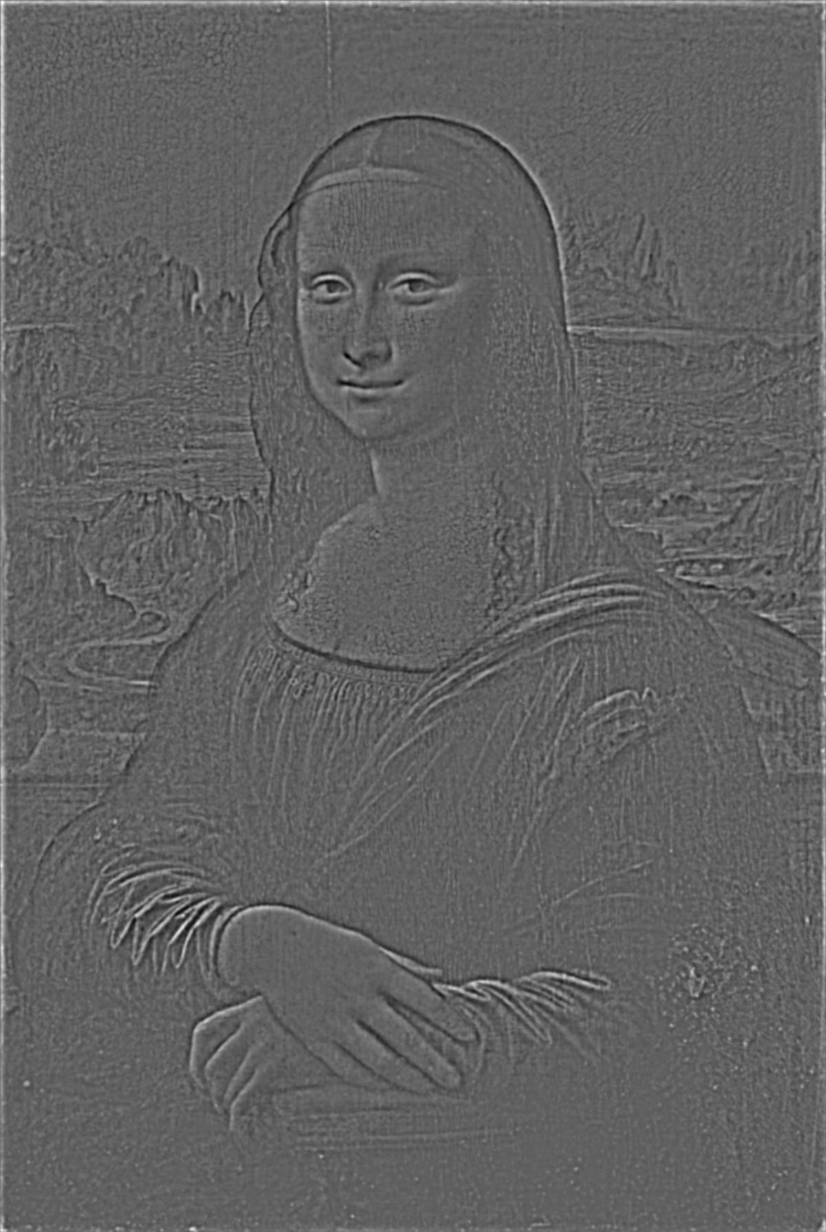
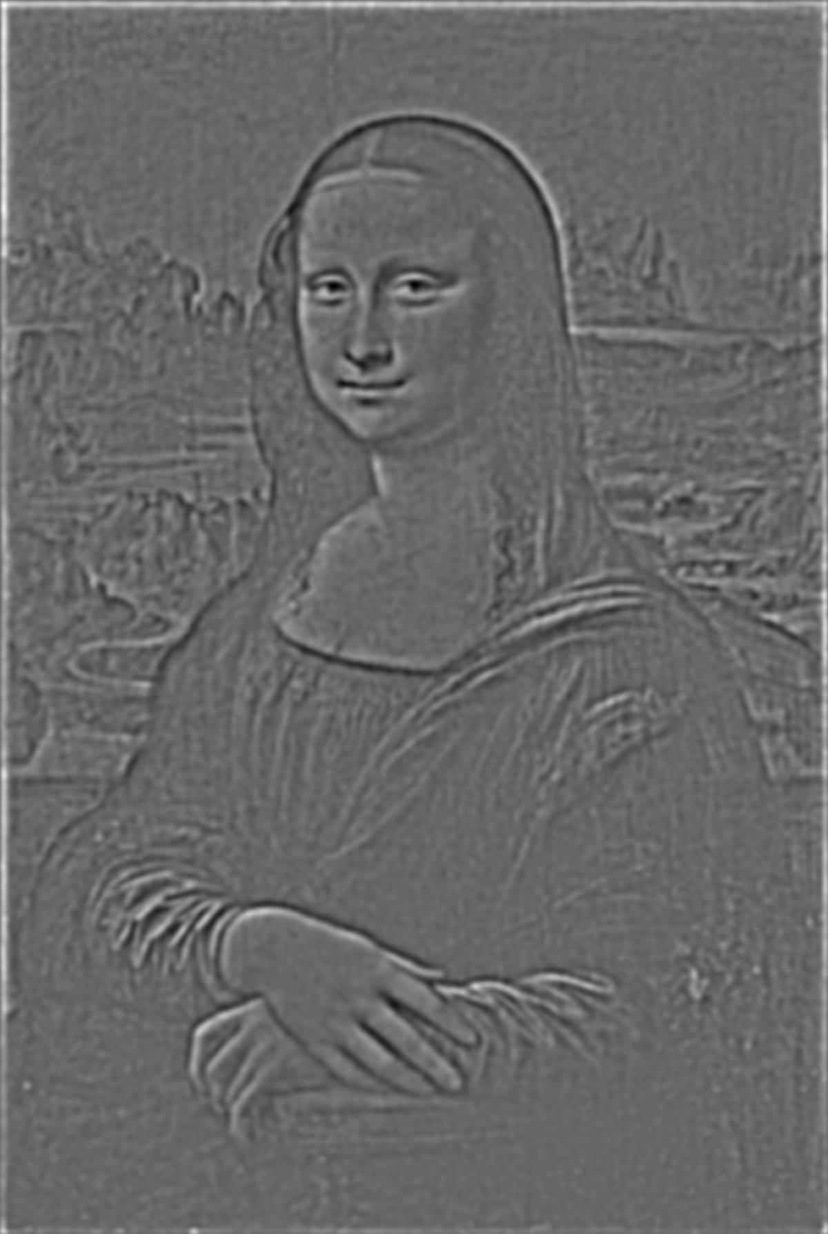
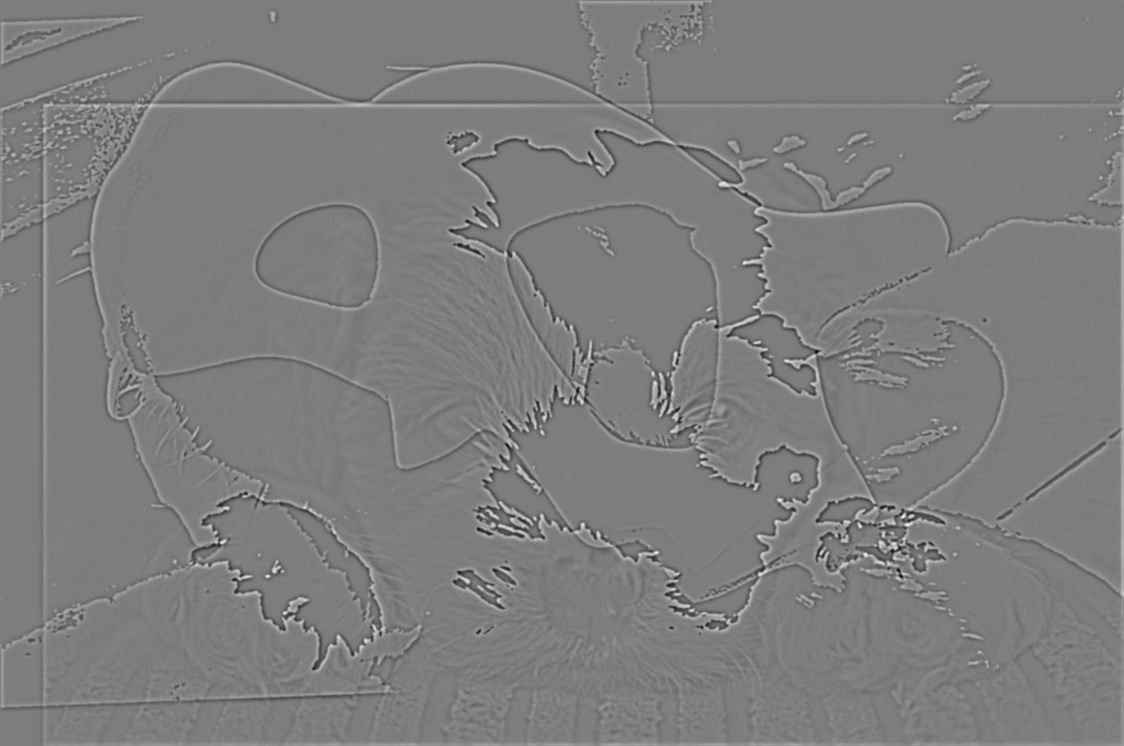
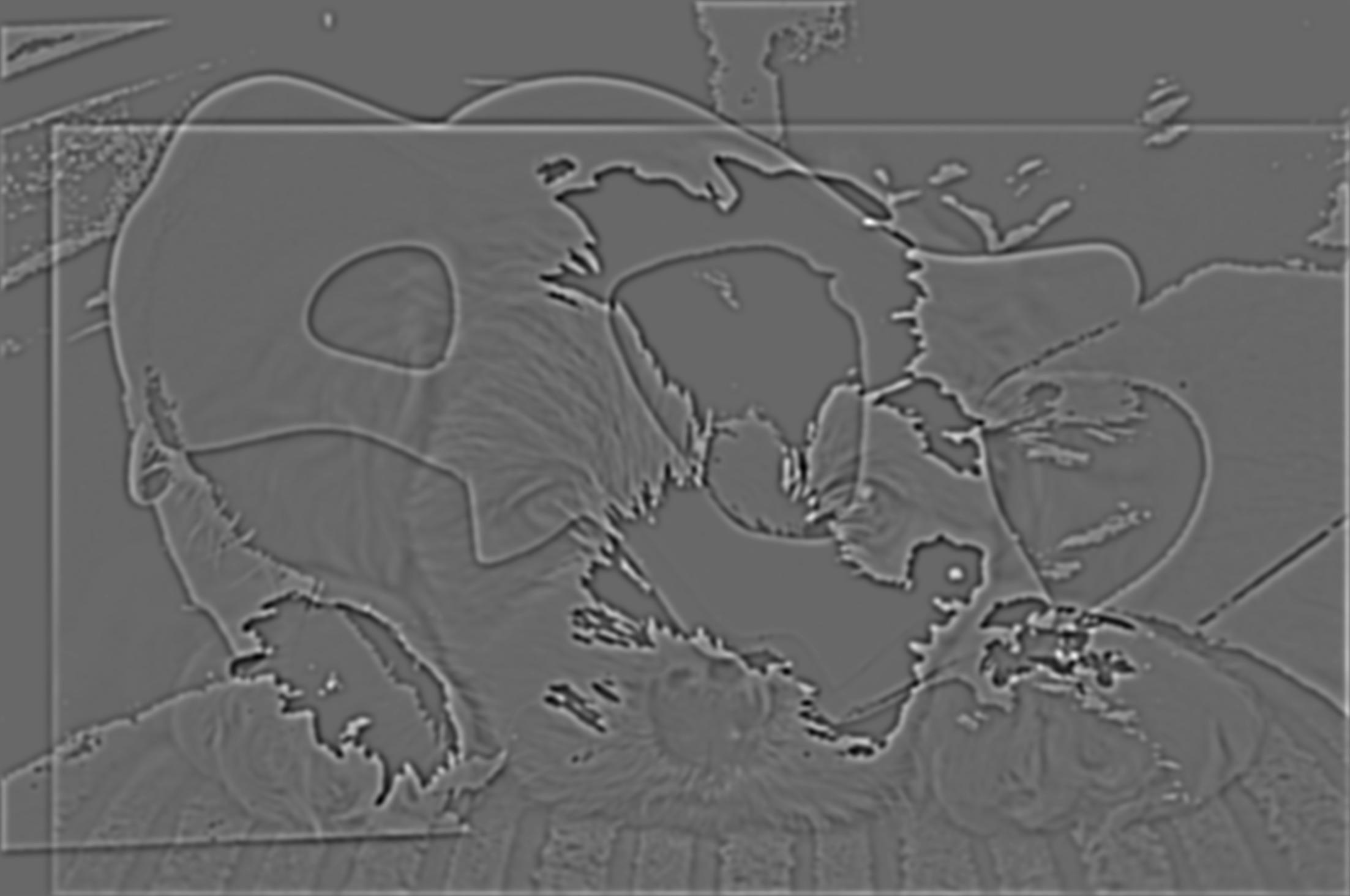
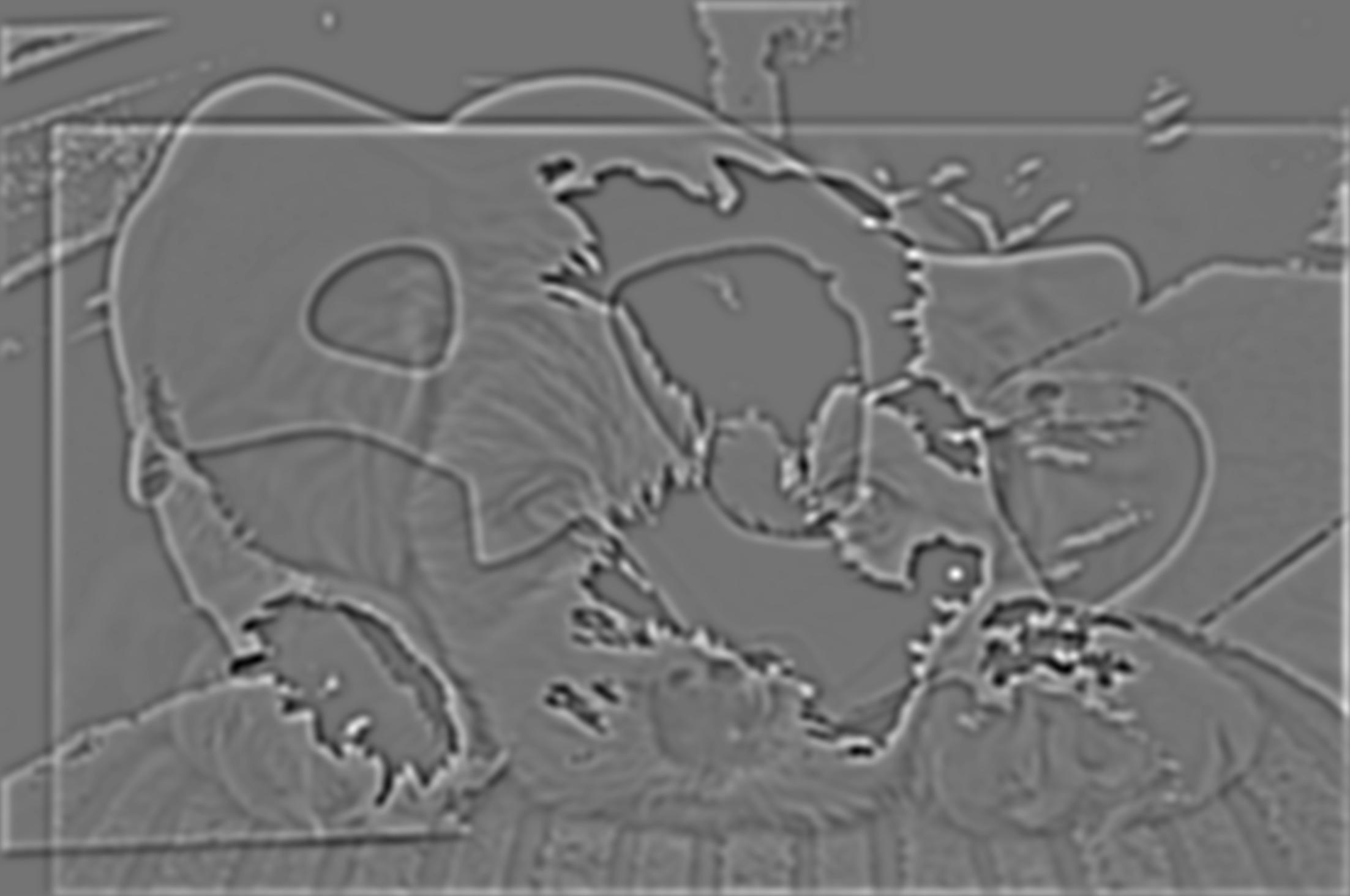
We can create the corresponding Laplacian stack where the $i'th$ image of the stack is the difference between the image $i$ and $i+1$ of the gaussian stack.
laplacian_stack = []
for i in range(5):
    dif = gaussian_stack[i] - gaussian_stack[i+1]
    laplacian_stack.append(dif)
    plt.imsave(f'l_lincoln_{i+1}.jpg', dif, cmap='gray')
laplacian_stack.append(gaussian_stack[-1])
plt.imsave(f'l_lincoln_{6}.jpg', blurred, cmap='gray')
Laplacian Stack of Lincoln in Dalivison
 |
 |
 |
 |
 |
 |
def create_stack(img_name, layers=6):
    img = skio.imread(img_name)
    img_name = img_name[:-4]
    gaussian_stack = []
    blurred = sc.rgb2gray(img)
    for i in range(1, 7):
        g_new = cv2.getGaussianKernel(ksize=20, sigma=2**i)
        g_new2d = g_new @ g_new.T
        blurred = convolve2d(blurred, g_new2d, mode='same')
        gaussian_stack.append(blurred)
        plt.imsave(f'{img_name}_{i}.jpg', blurred, cmap='gray')
    laplacian_stack = []
    for i in range(5):
        dif = gaussian_stack[i] - gaussian_stack[i+1]
        laplacian_stack.append(dif)
        plt.imsave(f'l_{img_name}_{i+1}.jpg', dif, cmap='gray')
    laplacian_stack.append(gaussian_stack[-1])
    plt.imsave(f'l_{img_name}_{6}.jpg', blurred, cmap='gray')

    return np.array(gaussian_stack), np.array(laplacian_stack)
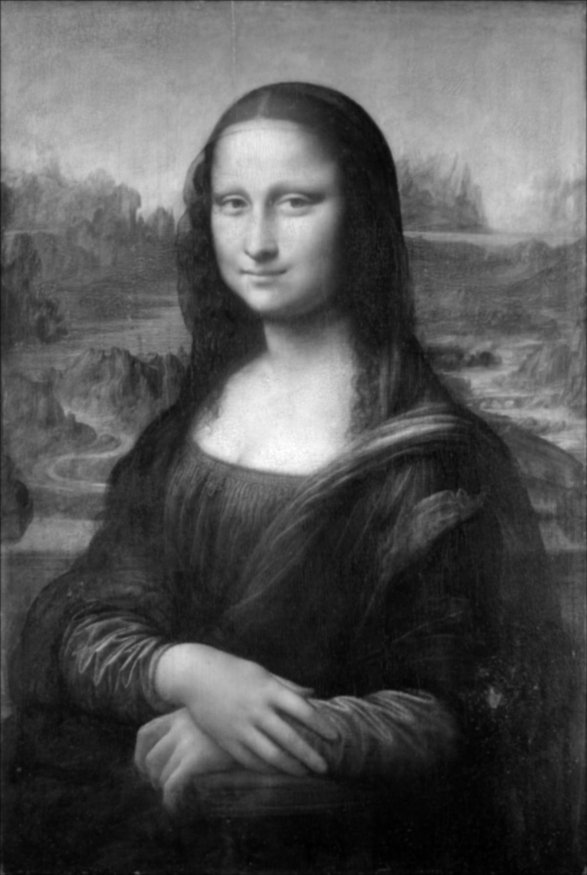
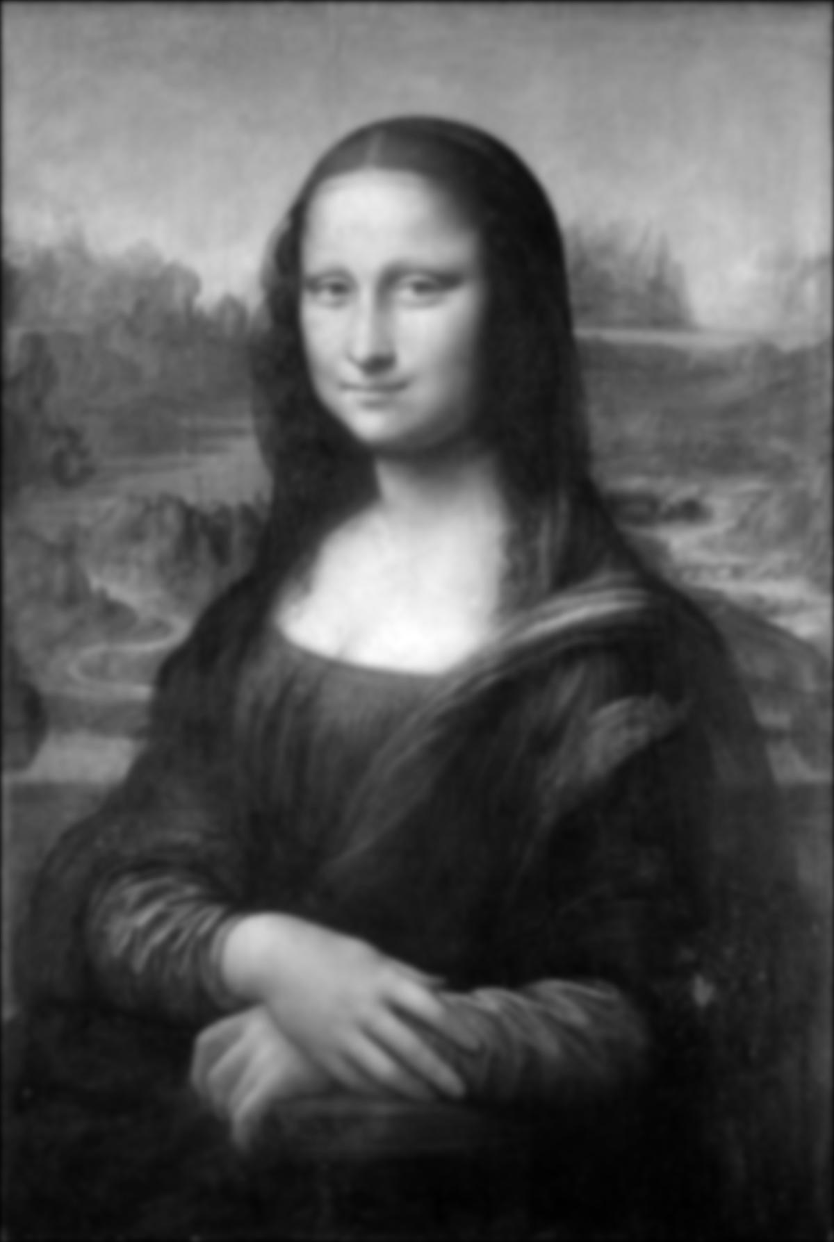
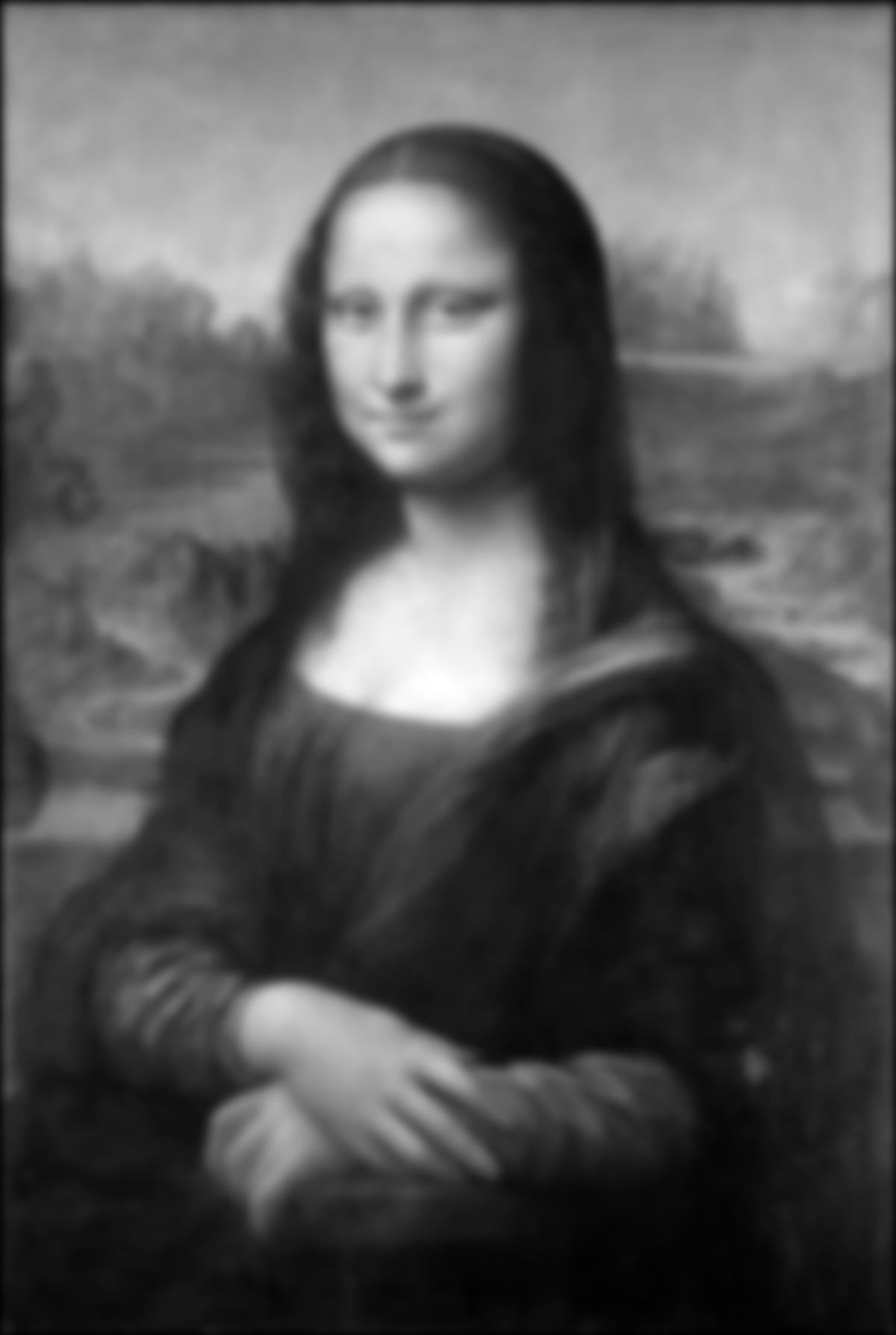
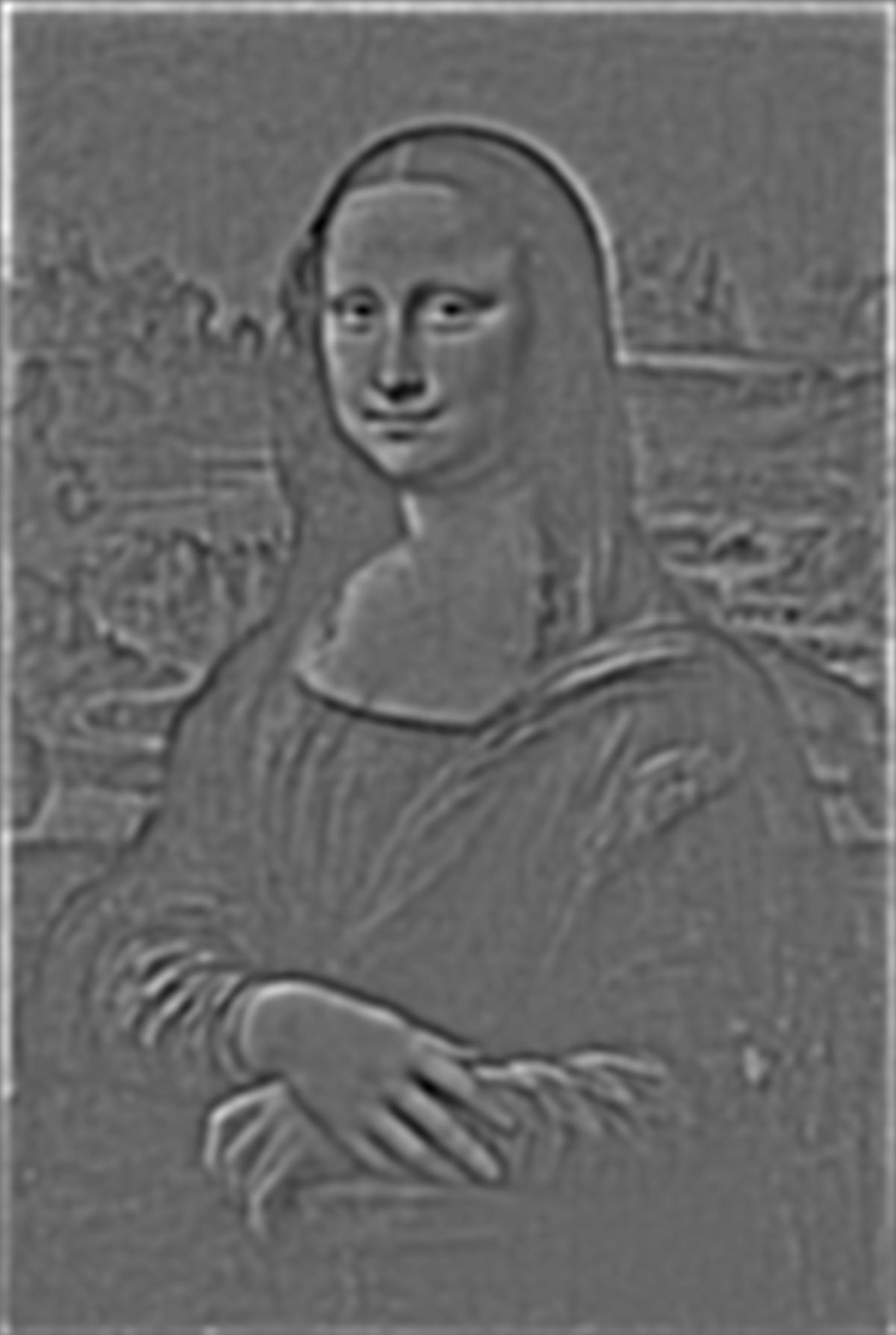
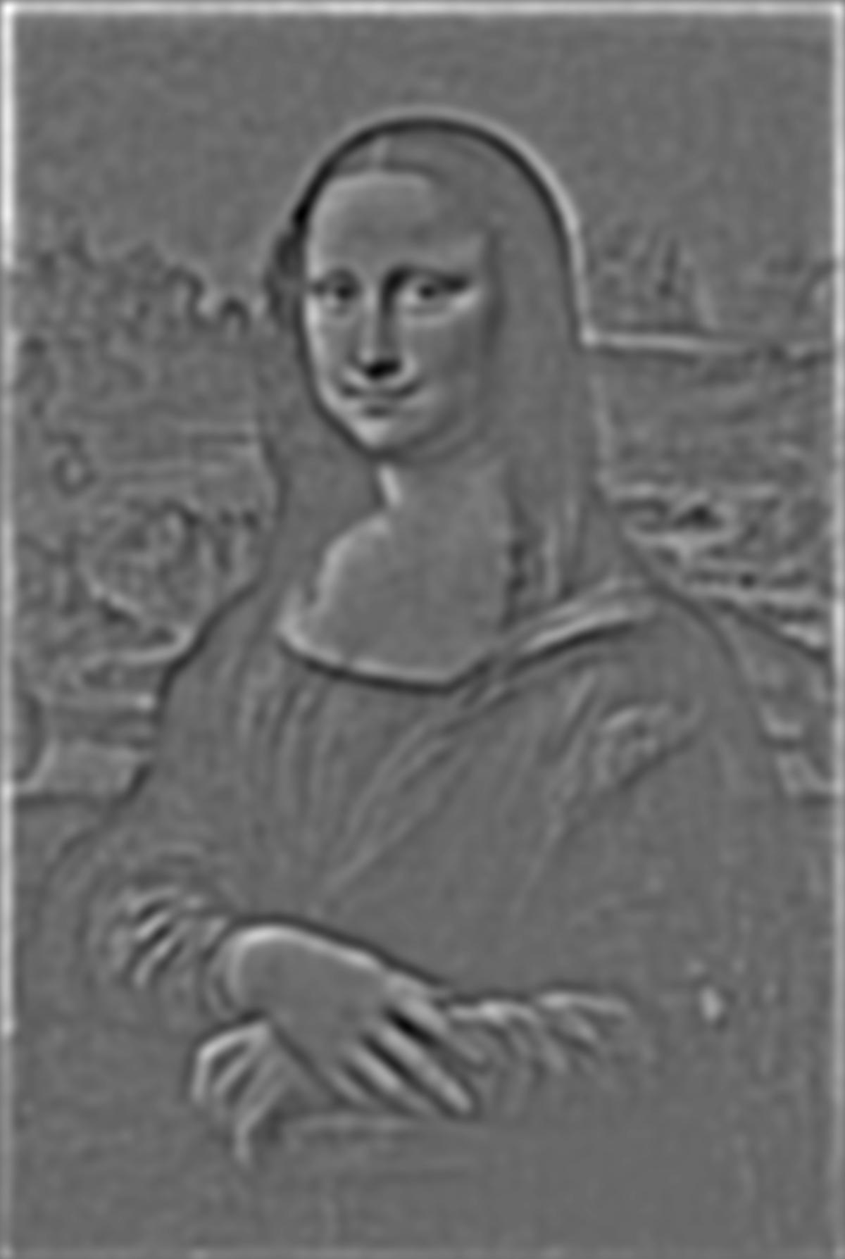
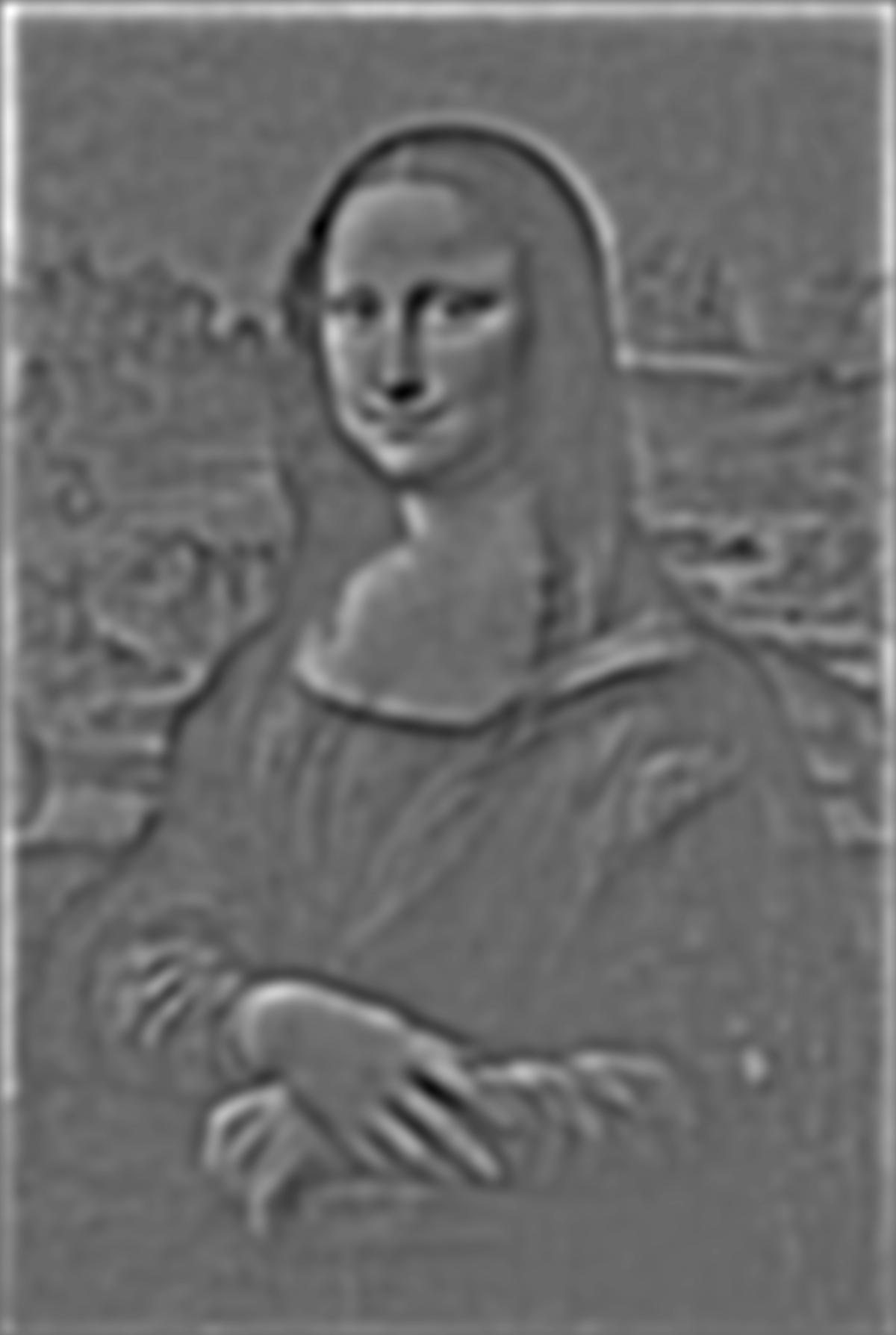
Gaussian & Laplacian Stacks of The Mona Lisa
create_stack('monalisa.jpg')
 |
 |
 |
 |
 |
 |
 |
 |
 |
 |
 |
 |
Gaussian and Laplacian Stacks of our adorable combined image from earlier
create_stack('puppy_cubone.jpg')
 |
 |
 |
 |
 |
 |
 |
 |
 |
 |
 |
 |
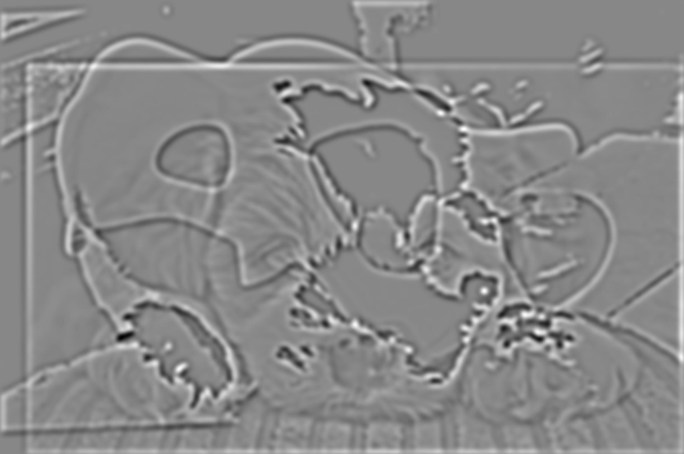
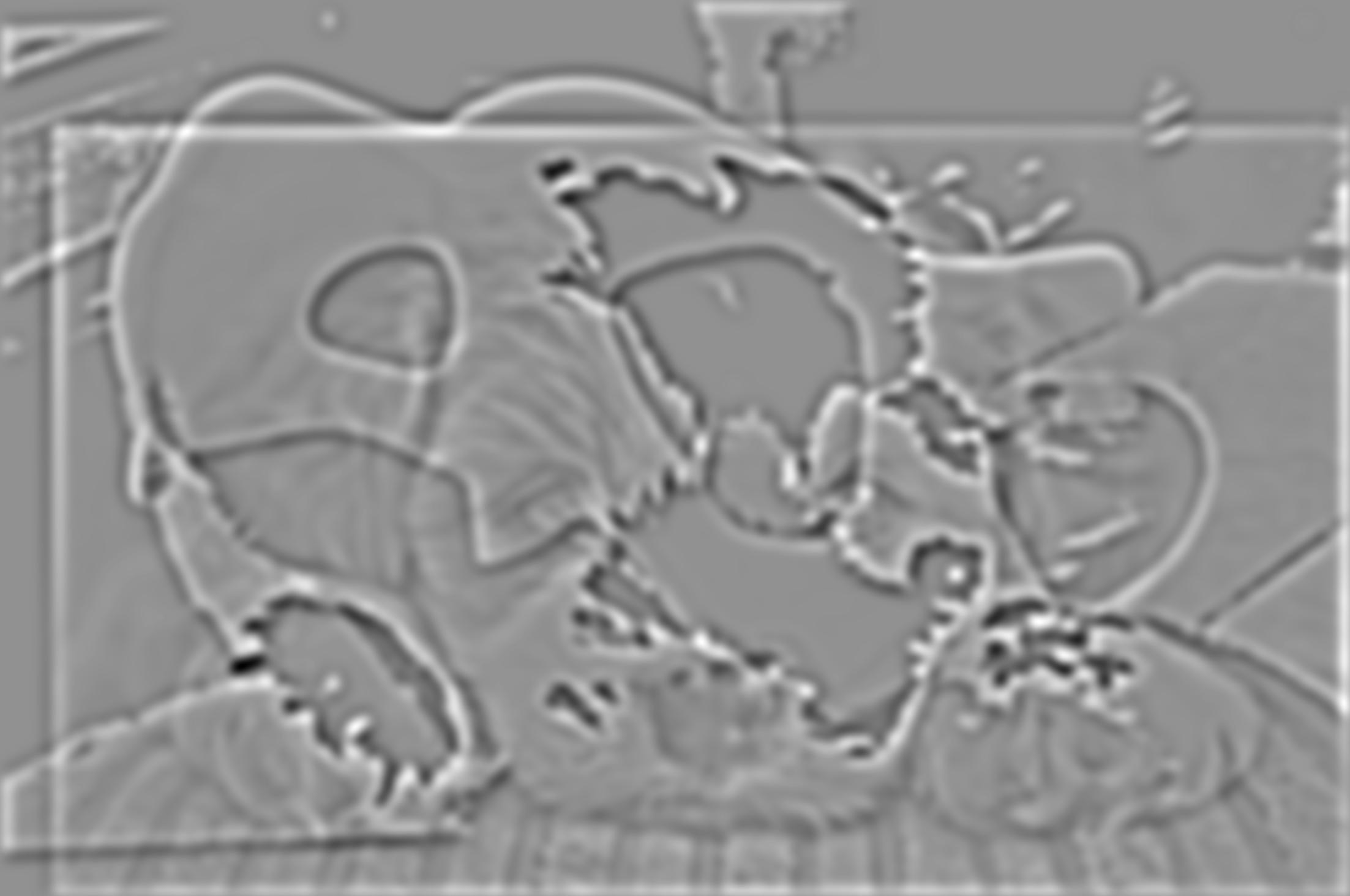
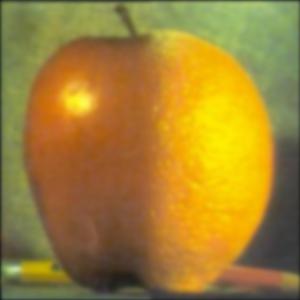
Part 2.4 Multiresolution Blending (a.k.a The Oraple!)
In the final part of the project, we attempt to blend images together by creating a combined laplacian stack between two images that is weighted by a predefined image mask. The precise algorithm is described below.
Laplacian Pyramid Blending Algorithm
- Build Laplacian stacks LA and LB for images A and B respectively
- Build Gaussian stacks GR for the region image R.
- Form a combined stack LS from LA and LB using nodes of GR as weights. That is, for each $l$, $i$, and $j$: $LS_l(i, j) = GR_l(i, j)LA_l(i,j) + (1-GR_l(i,j))LB_l(i,j)$
- Obtain the splined image S by expanding and summing the levels of LS
def create_stack_b(img_name, layers=6):
    blurred = img_name
    gaussian_stack = []
    for i in range(1, 7):
        g_new = cv2.getGaussianKernel(ksize=20, sigma=2**i)
        g_new2d = g_new @ g_new.T
        blurred = convolve2d(blurred, g_new2d, mode='same')
        gaussian_stack.append(blurred)
    laplacian_stack = []
    for i in range(5):
        dif = gaussian_stack[i] - gaussian_stack[i+1]
        laplacian_stack.append(dif)
    laplacian_stack.append(gaussian_stack[-1])

    return np.array(gaussian_stack), np.array(laplacian_stack)
def blend_image(img1, img2, mask):
    GAr, LAr = create_stack_b(img1[:, :, 0])
    GAg, LAg = create_stack_b(img1[:, :, 1])
    GAb, LAb = create_stack_b(img1[:, :, 2])
    GBr, LBr = create_stack_b(img2[:, :, 0])
    GBg, LBg = create_stack_b(img2[:, :, 1])
    GBb, LBb = create_stack_b(img2[:, :, 2])
    GR, LR = create_stack_b(mask)

    LSr = GR*LAr + (1-GR)*LBr
    LSg = GR*LAg + (1-GR)*LBg
    LSb = GR*LAb + (1-GR)*LBb

    LS = np.dstack((np.sum(LSr, axis=0), np.sum(LSg, axis=0), np.sum(LSb, axis=0)))
    skio.imsave('blended_image_3.jpg', LS)
    skio.imshow(LS/255)
def get_laplacians(img1, img2, mask):
    GAr, LAr = create_stack_b(img1[:, :, 0])
    GAg, LAg = create_stack_b(img1[:, :, 1])
    GAb, LAb = create_stack_b(img1[:, :, 2])
    GBr, LBr = create_stack_b(img2[:, :, 0])
    GBg, LBg = create_stack_b(img2[:, :, 1])
    GBb, LBb = create_stack_b(img2[:, :, 2])
    GR, LR = create_stack_b(mask)

    LSr = GR*LAr + (1-GR)*LBr
    LSg = GR*LAg + (1-GR)*LBg
    LSb = GR*LAb + (1-GR)*LBb

    for i in range(6):
        LA_i = np.dstack((LAr[i], LAg[i], LAb[i]))
        LB_i = np.dstack((LBr[i], LBg[i], LBb[i]))
        LS_i = np.dstack((LSr[i], LSg[i], LSb[i]))
        skio.imsave(f'LA_{i}.jpg', LA_i)
        skio.imsave(f'LB_{i}.jpg', LB_i)
        skio.imsave(f'LS_{i}.jpg', LS_i)
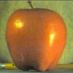
apple = skio.imread('apple.jpeg')
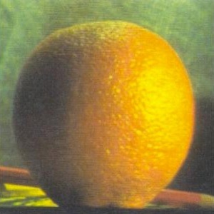
orange = skio.imread('orange.jpeg')
left_mask = np.zeros((300, 300))
left_mask[0:300, 0:150] = 1
plt.imsave('left_mask.jpg', left_mask, cmap='gray')
# blend_image(apple, orange, left_mask)
The Oraple
 |
 |
 |
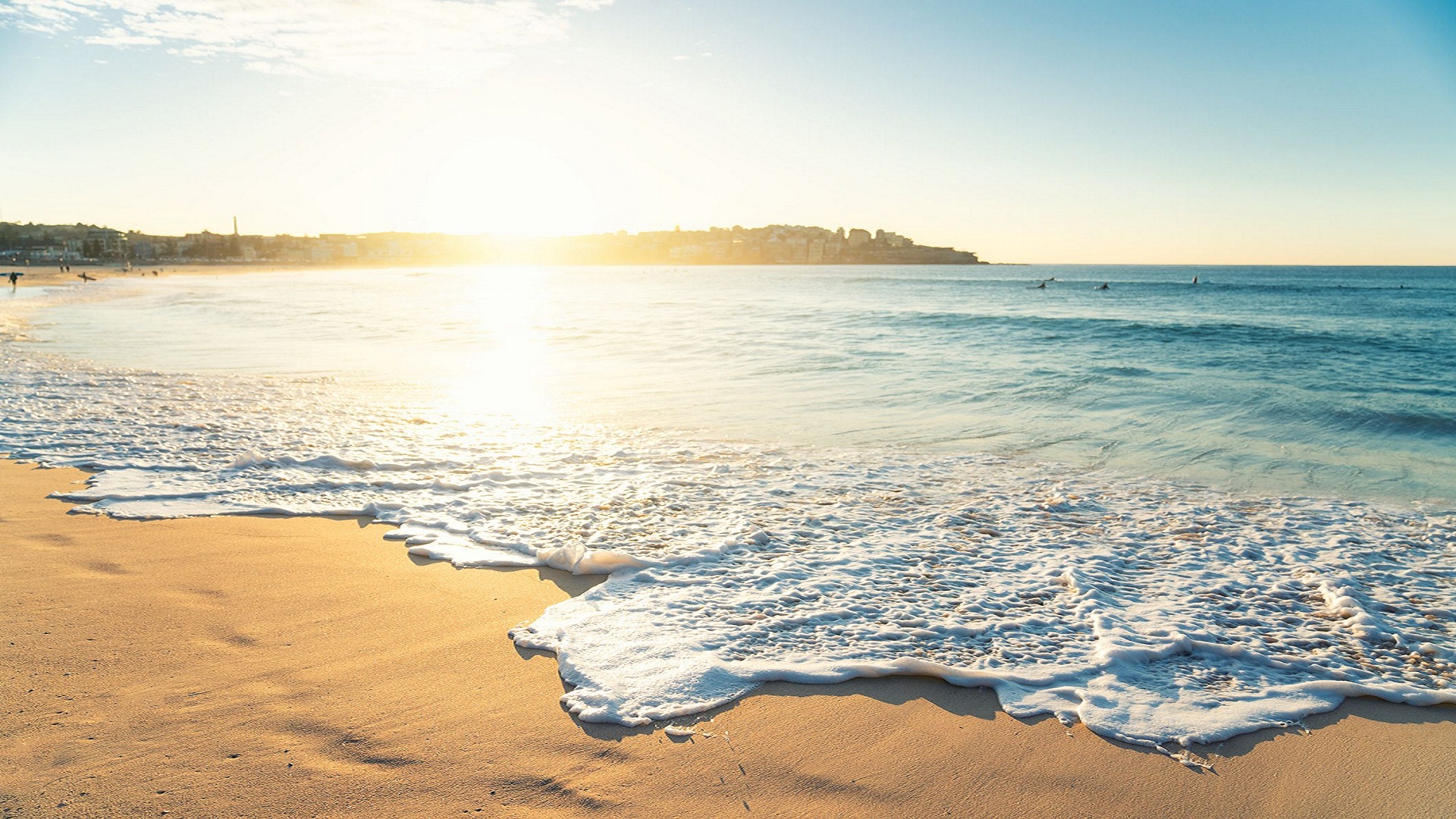
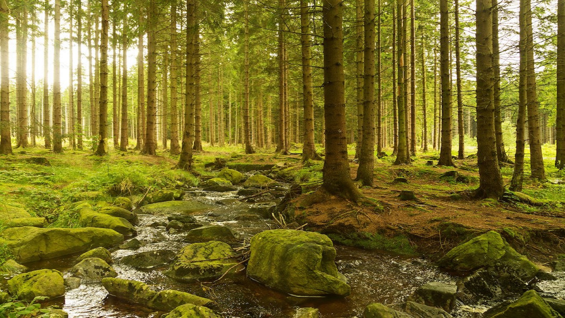
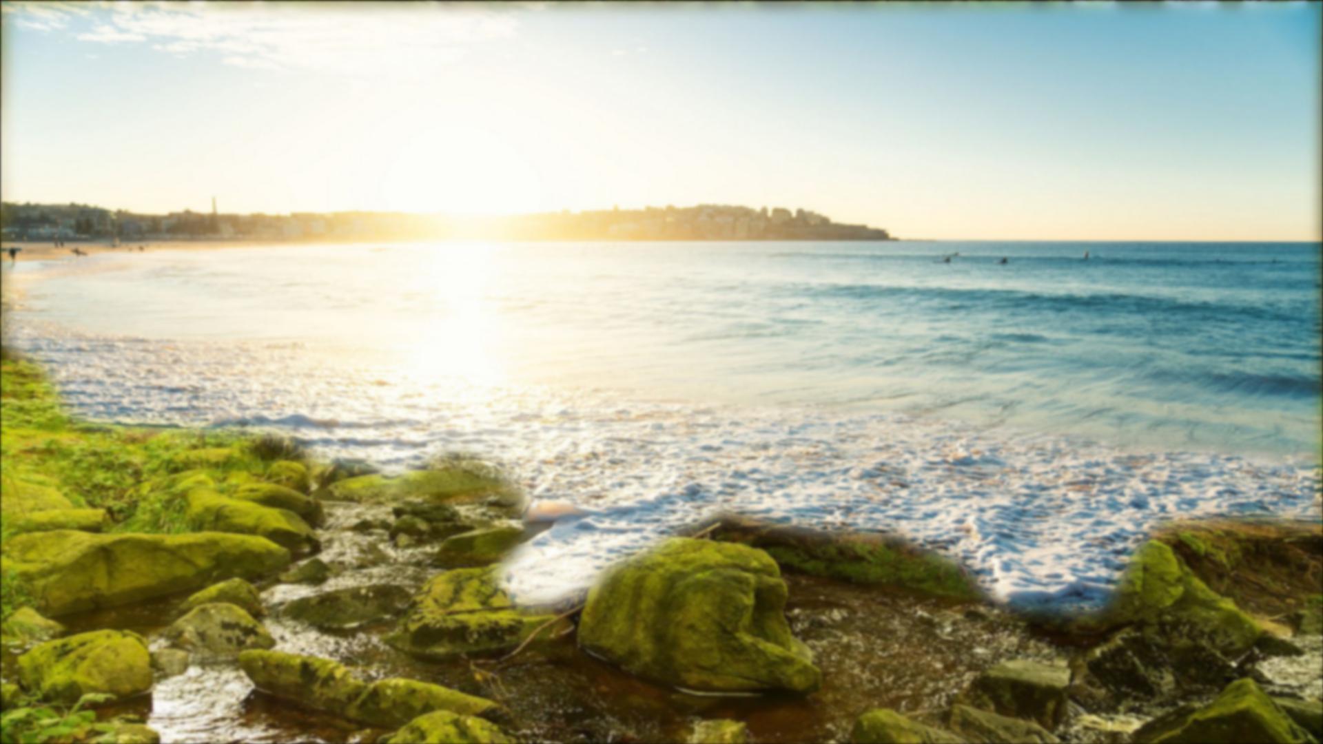
beach = skio.imread('beach.jpg')
forest = skio.imread('forest.jpg')
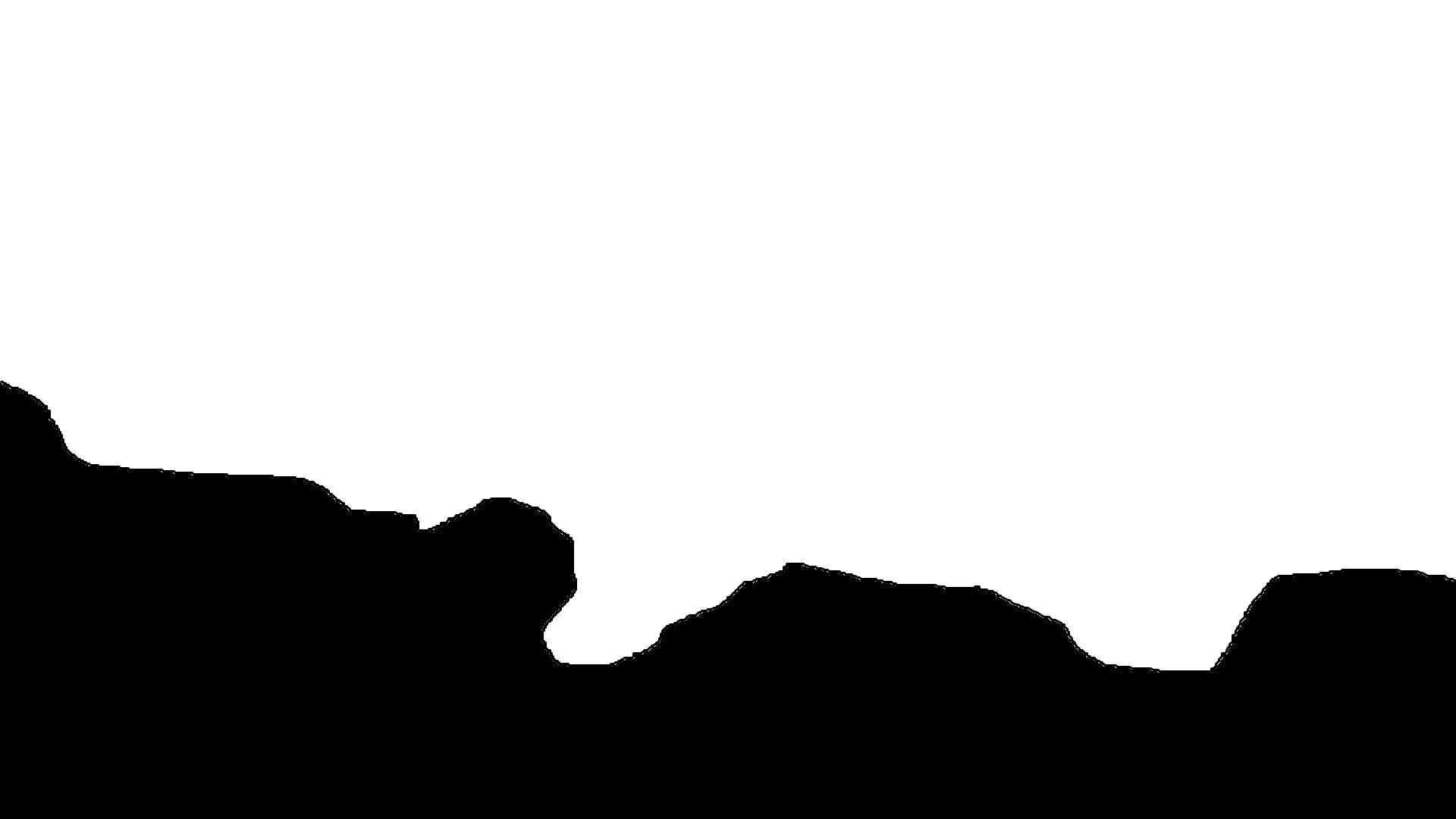
custom_mask = skio.imread('custom_mask2.jpg', as_gray=True)
# skio.imshow(beach)
# skio.imshow(forest)
# skio.imshow(custom_mask)
# blend_image(beach, forest, custom_mask)
Sunny beach and vibrant forest
 |
 |
 |
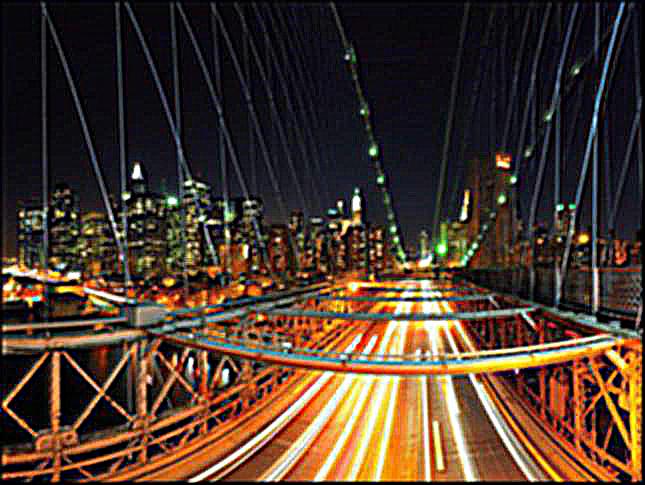
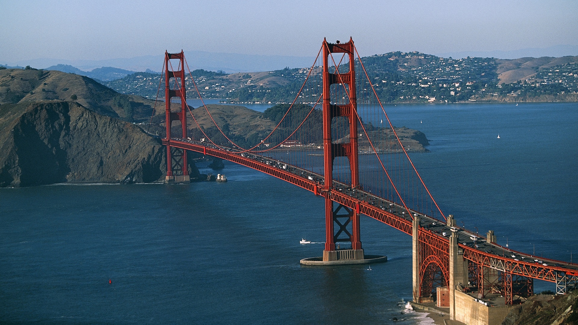
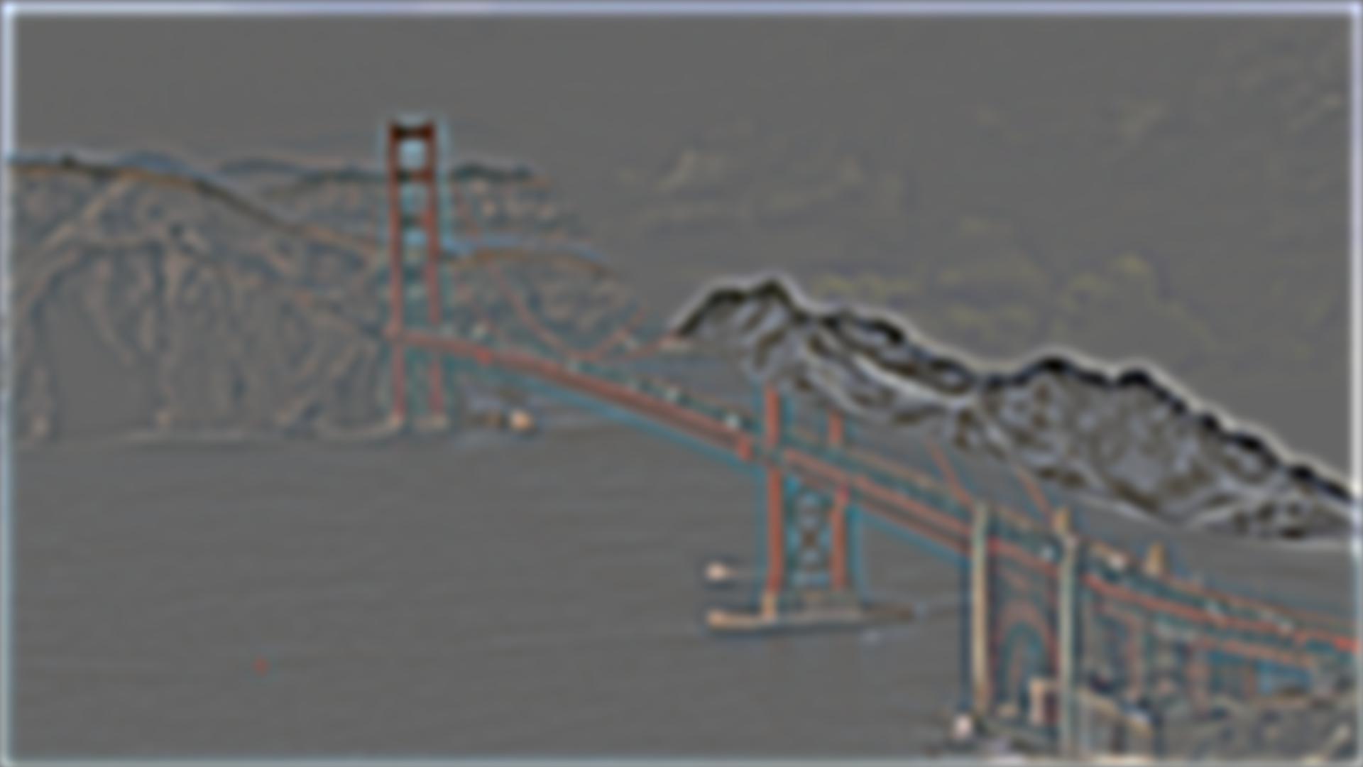
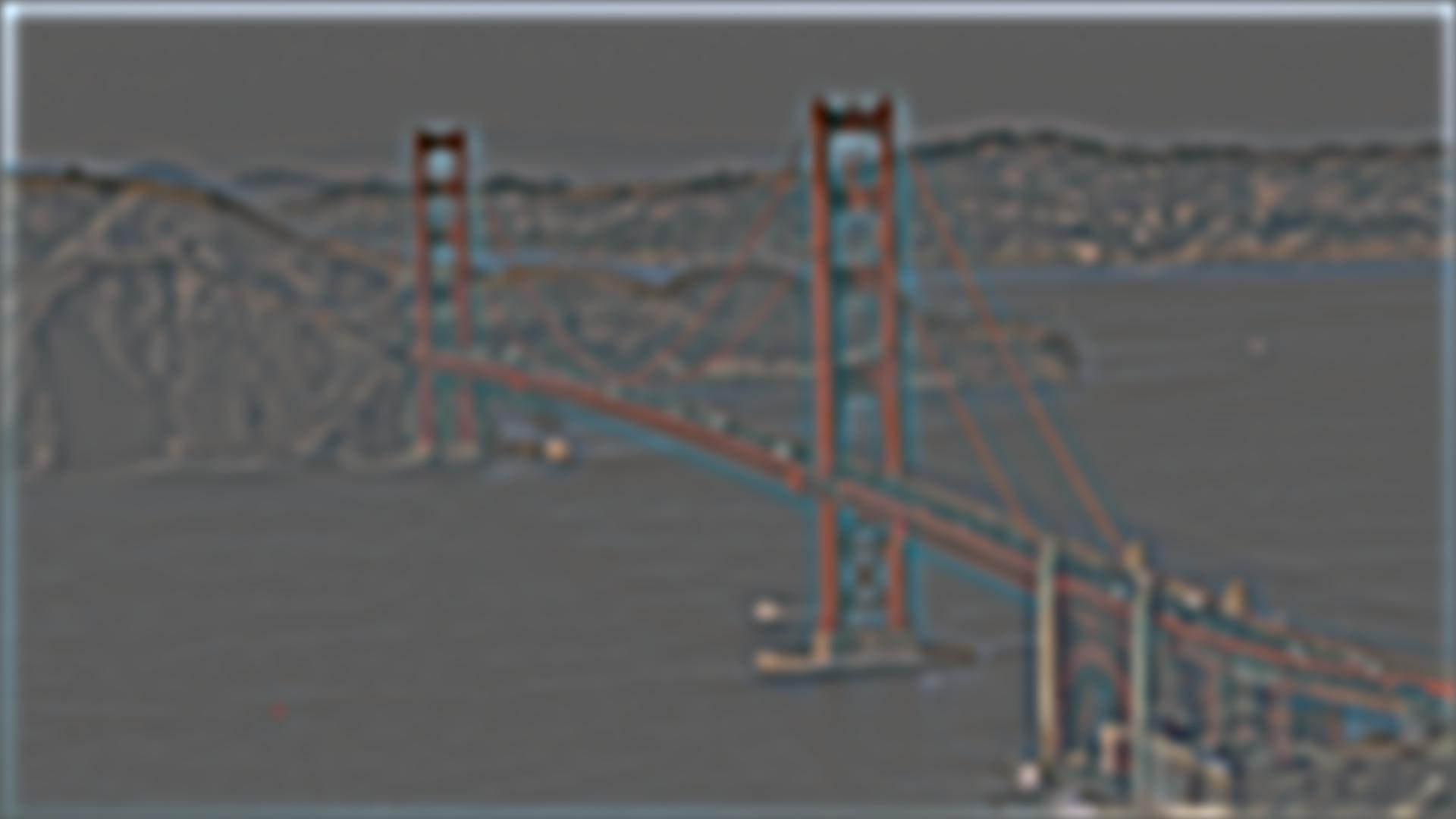
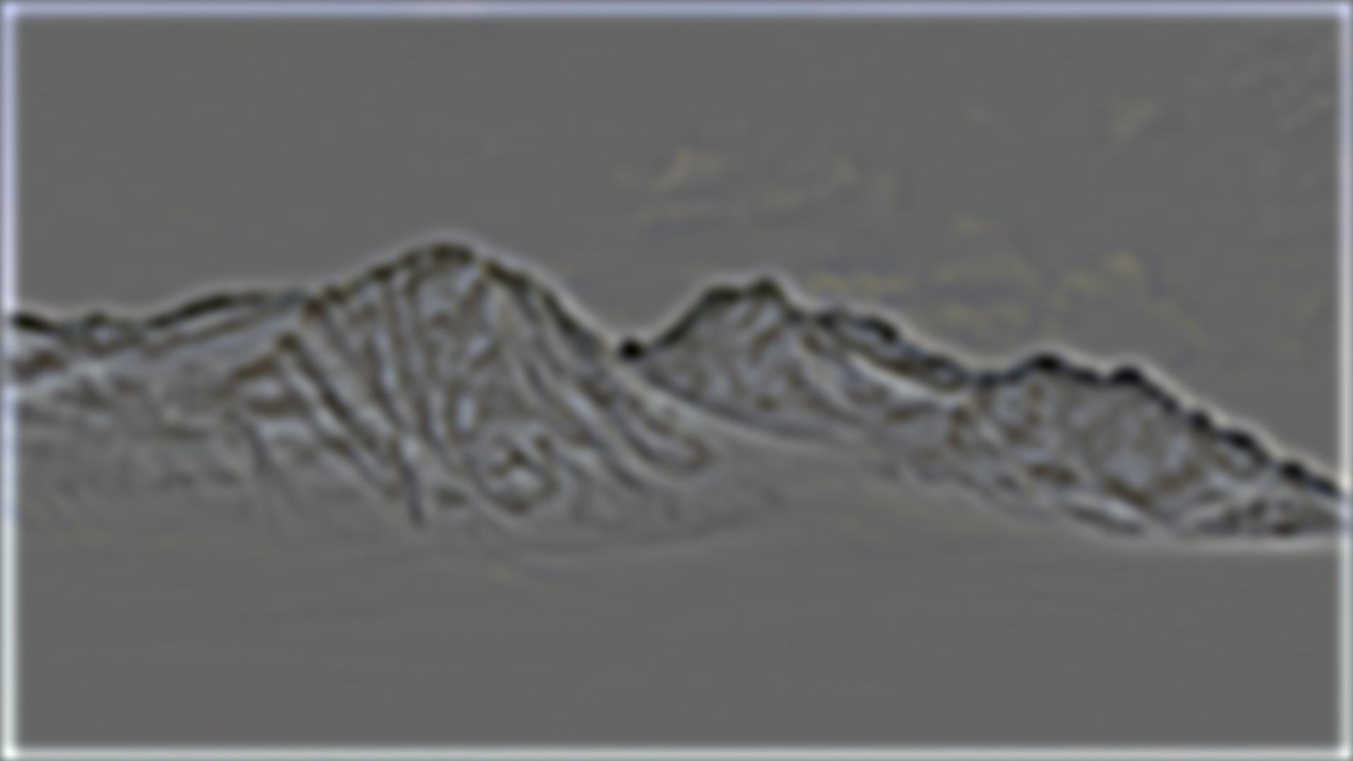
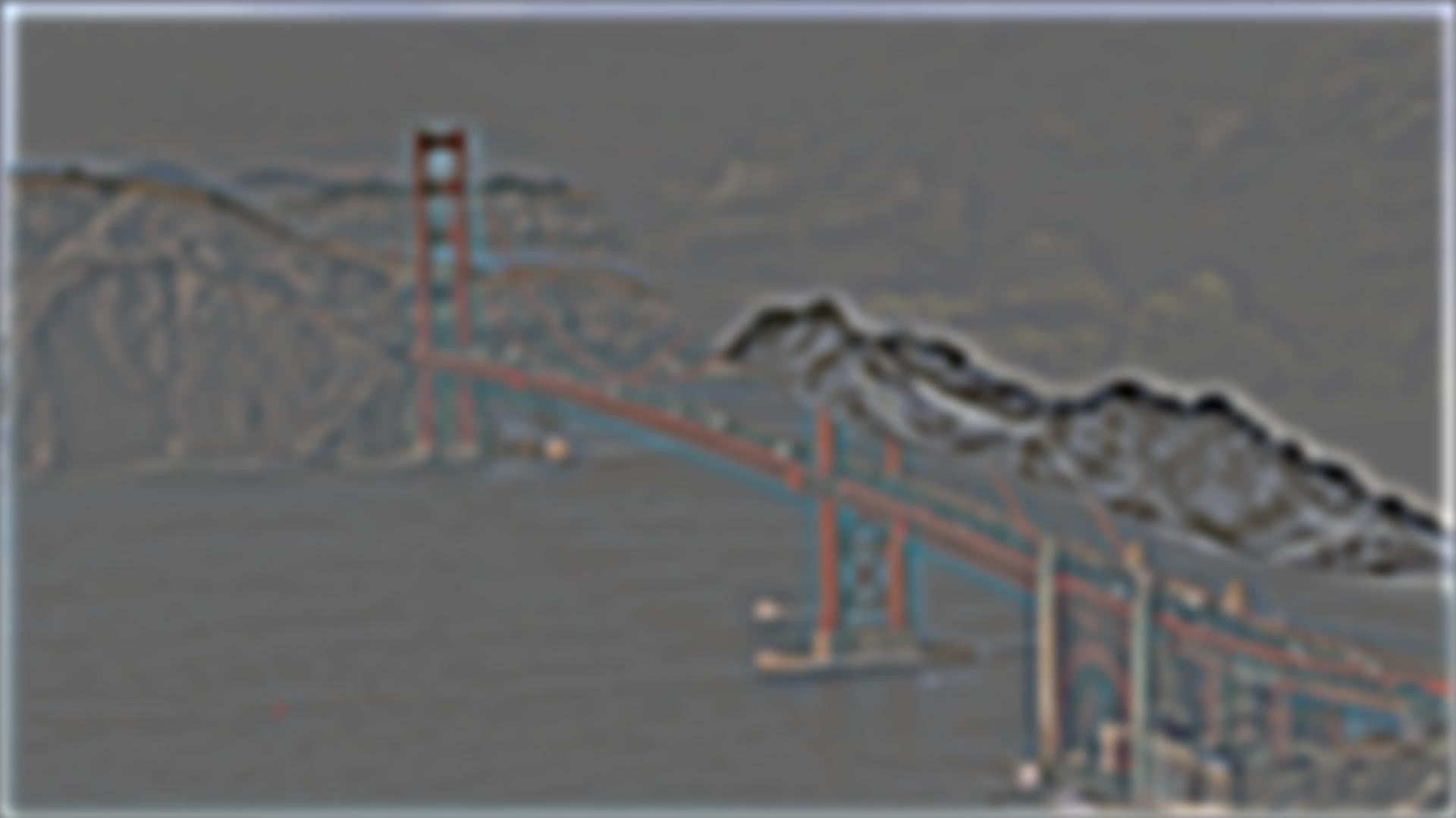
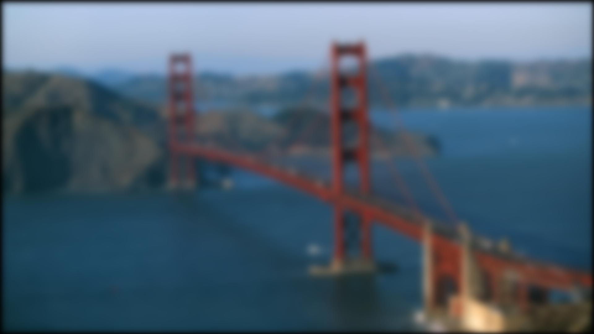
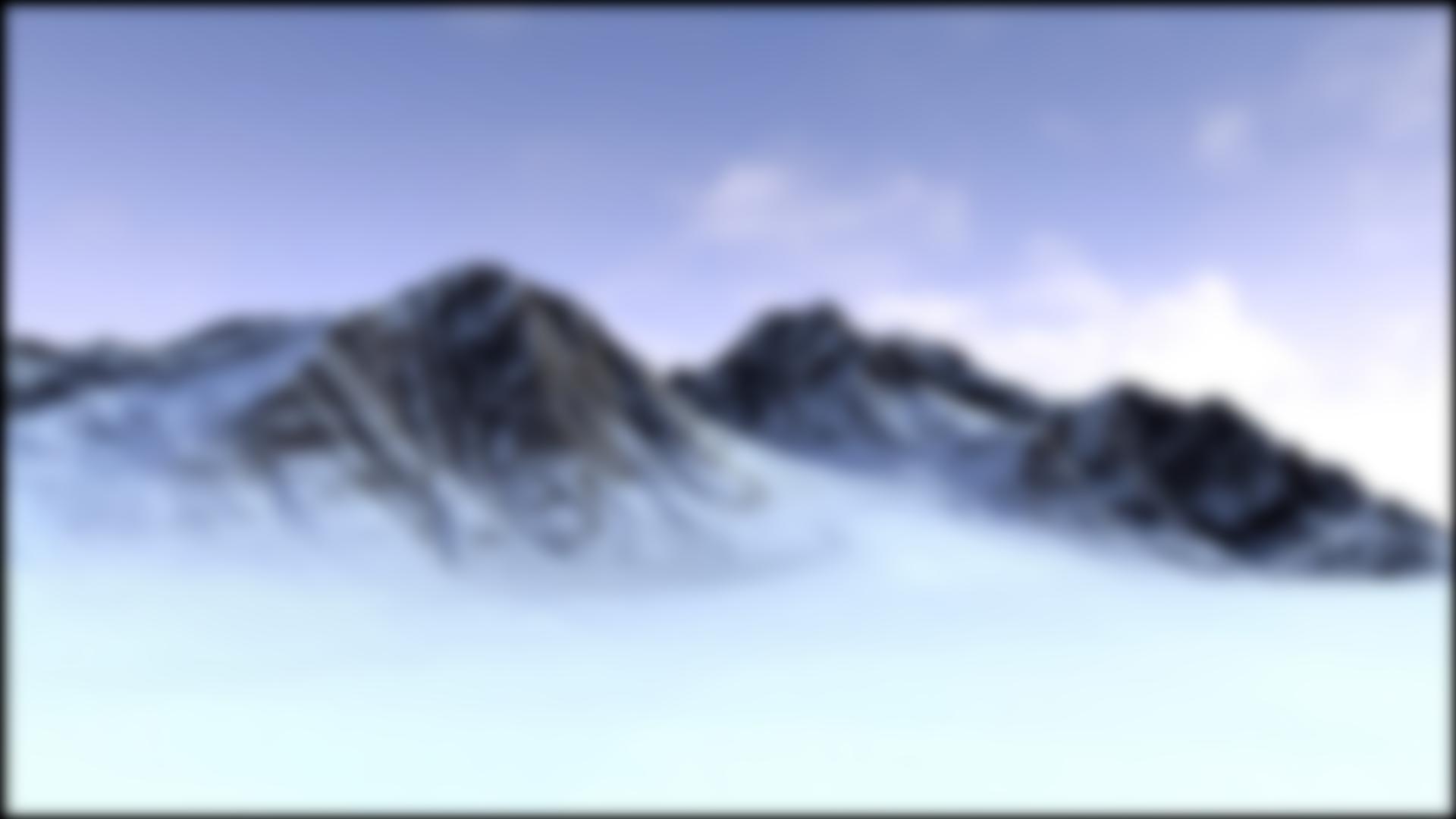
bridge = skio.imread('ggbridge.jpg')
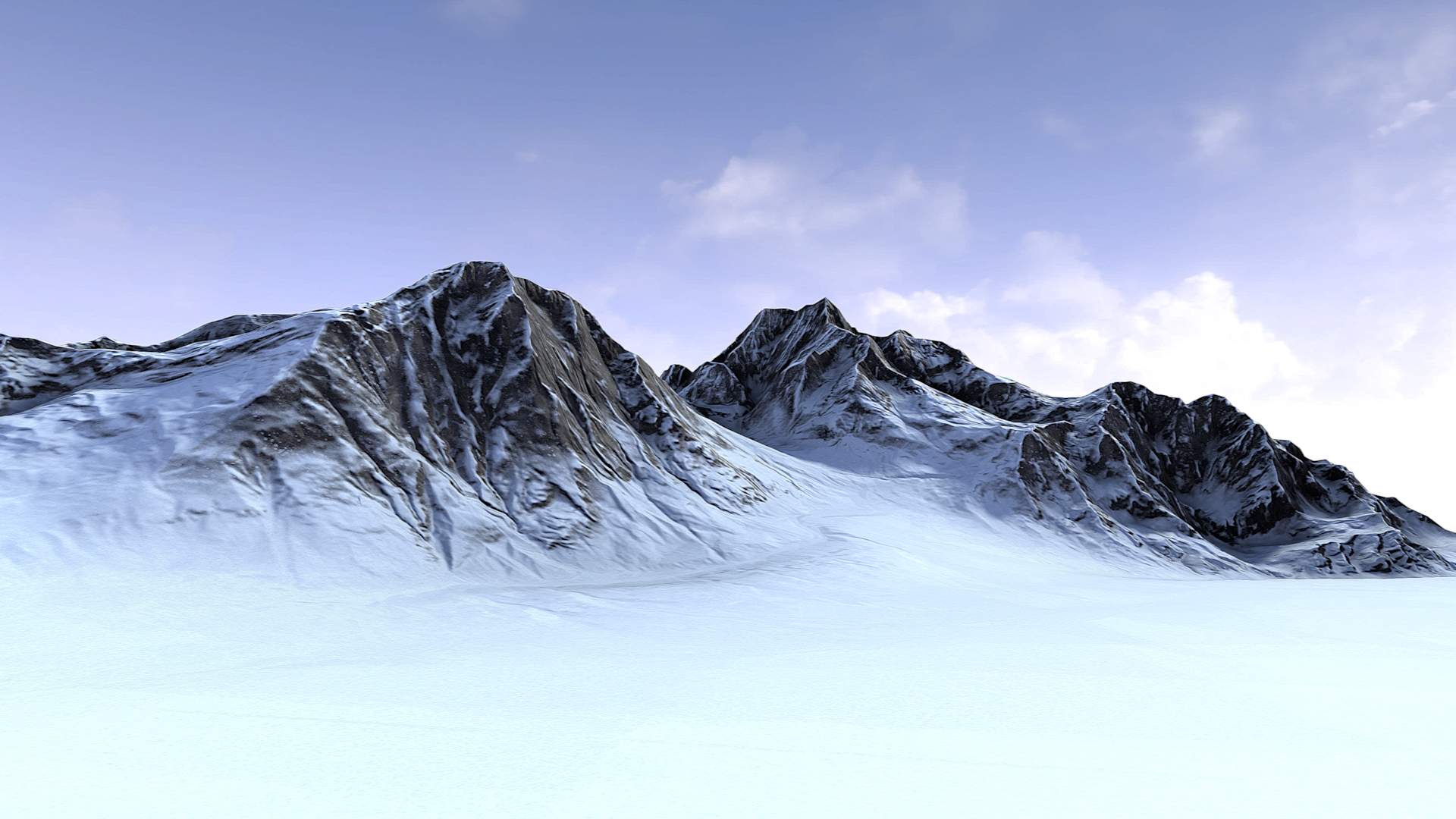
snow = skio.imread('snow.jpg')
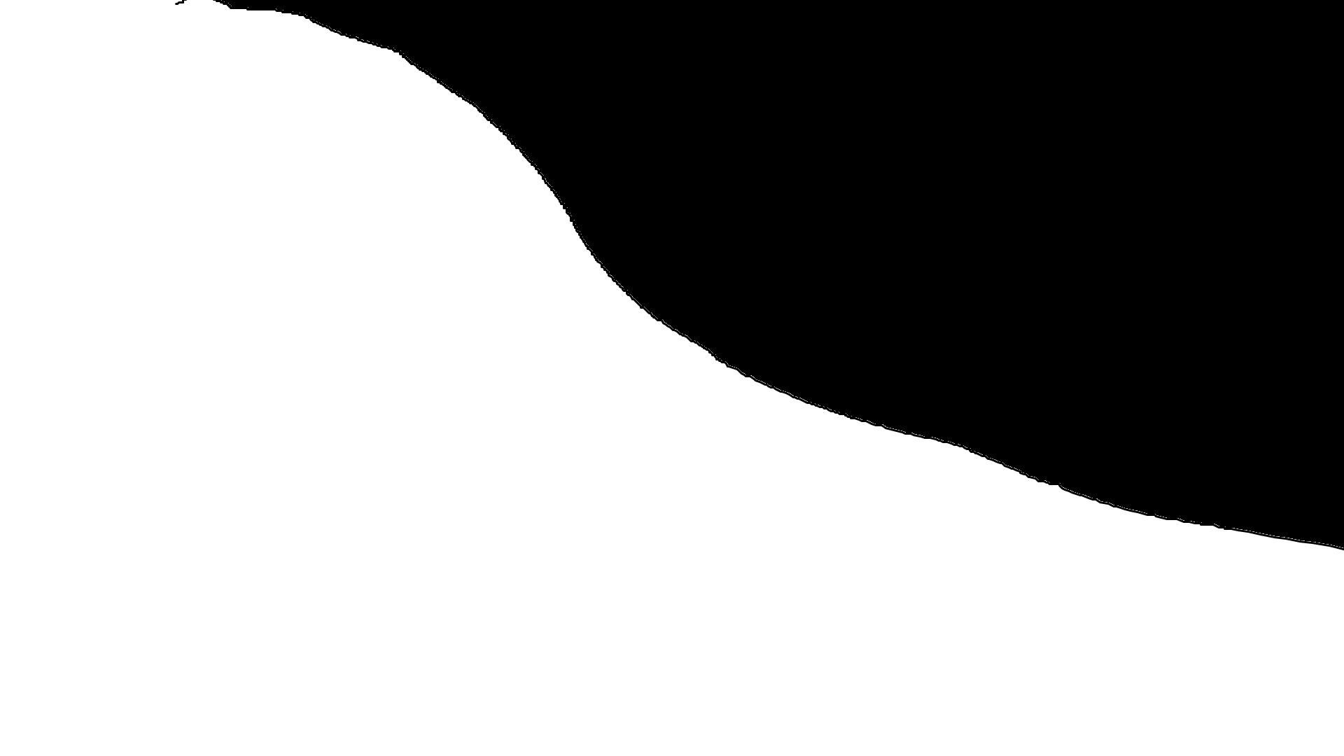
custom_mask = skio.imread('custom_blend.jpg', as_gray=True)
# skio.imshow(bridge)
# skio.imshow(snow)
# skio.imshow(custom_mask)
# blend_image(bridge, snow, custom_mask)
# get_laplacians(bridge, snow, custom_mask)
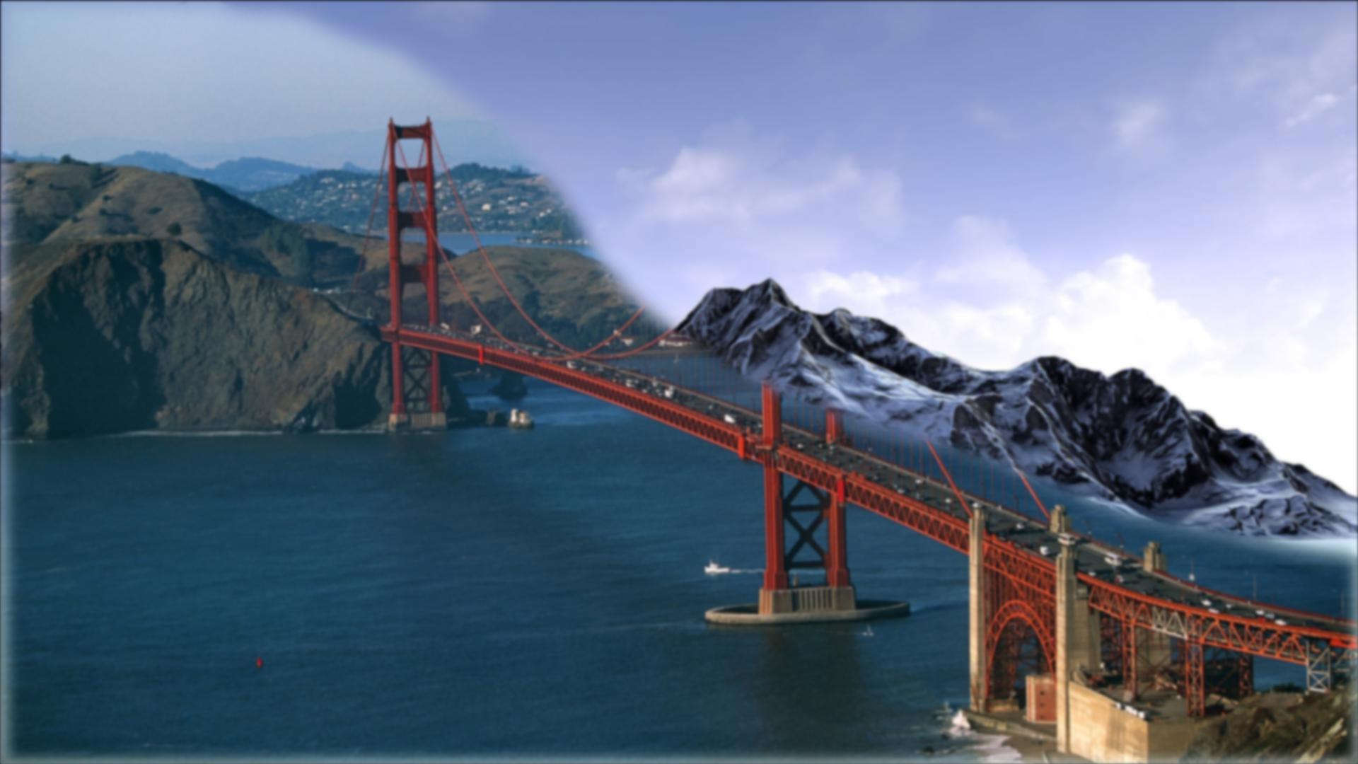
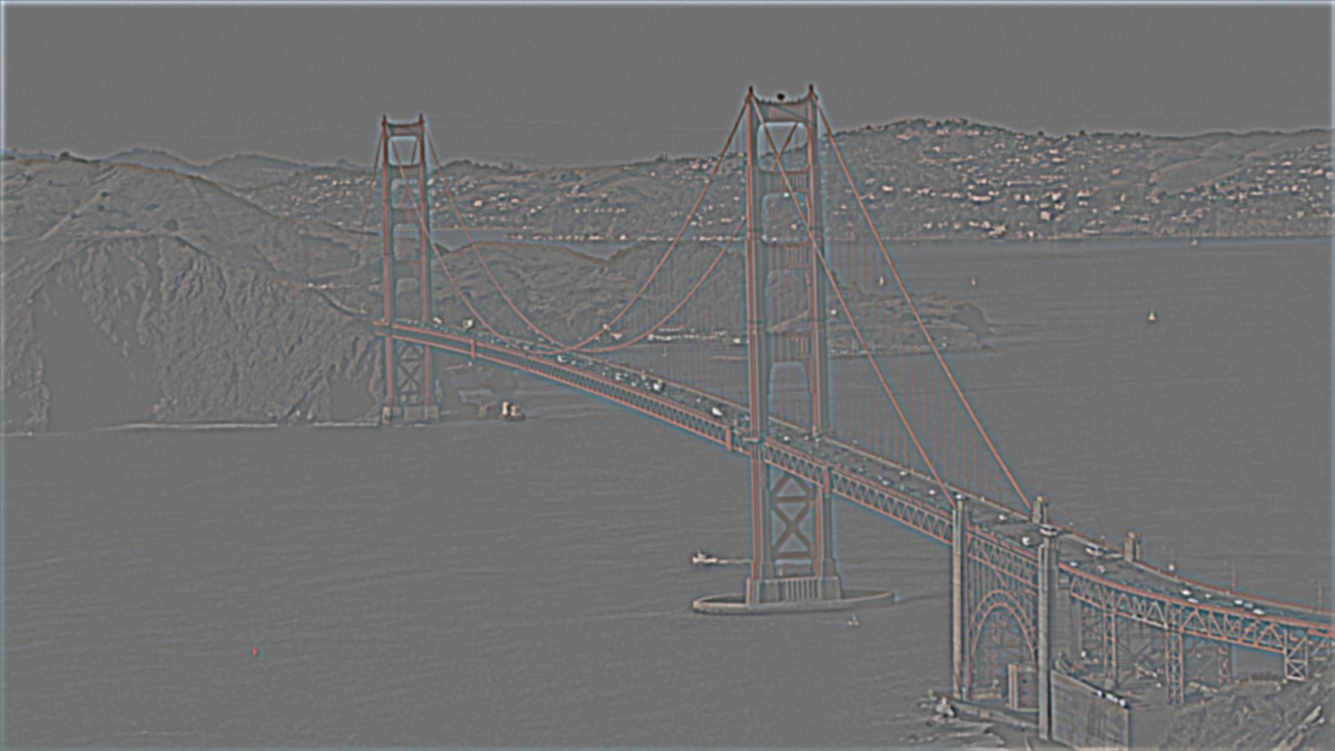
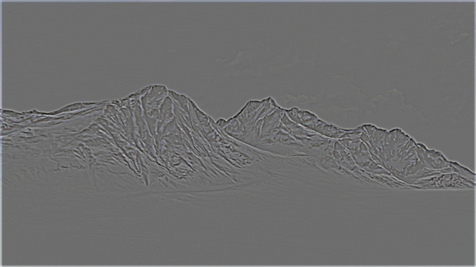
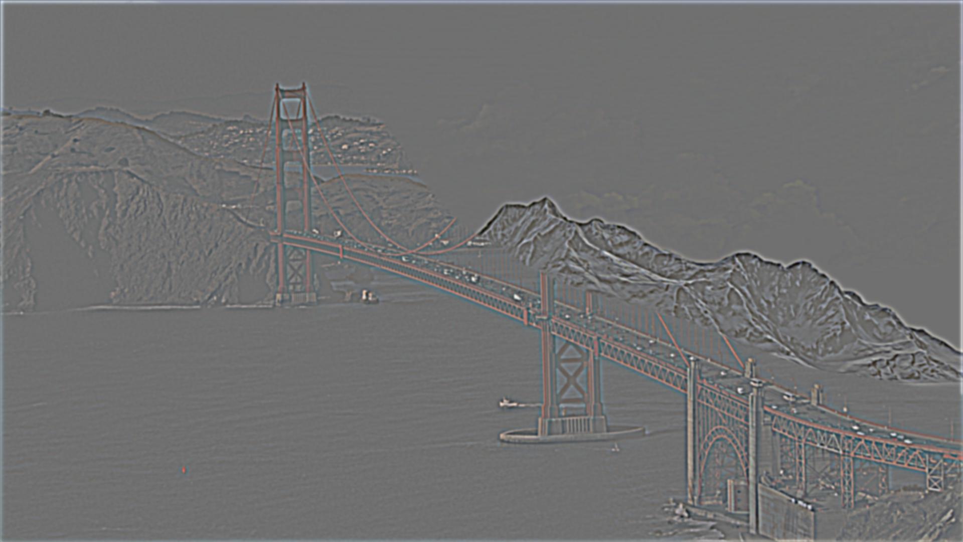
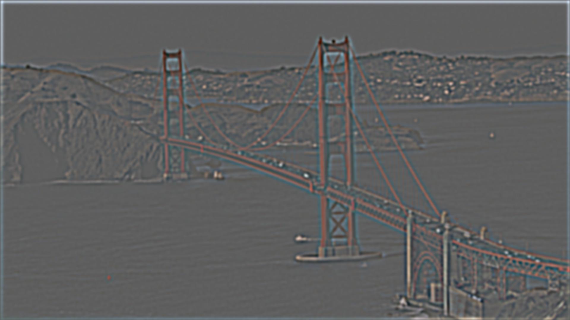
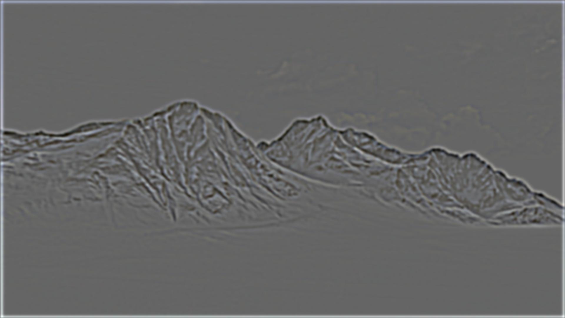
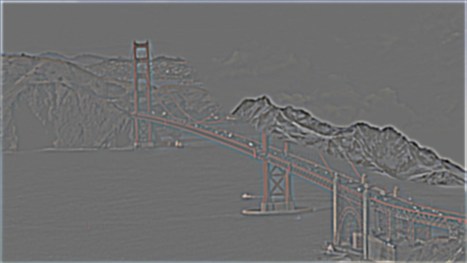
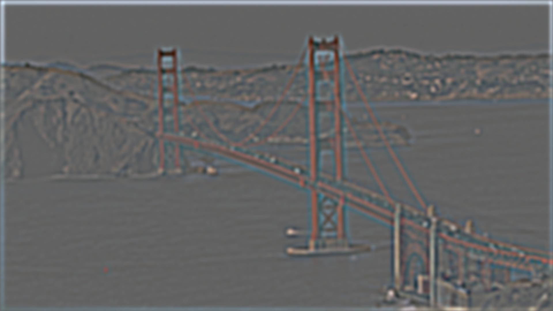
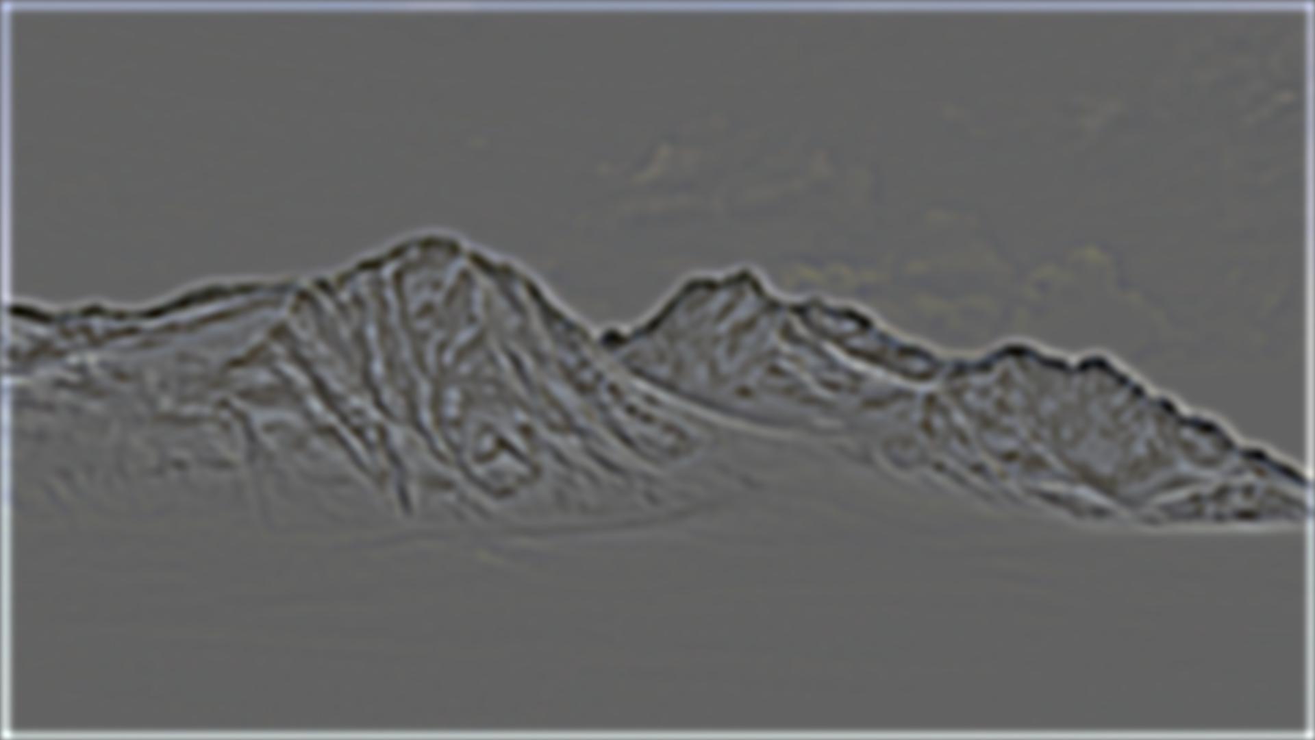
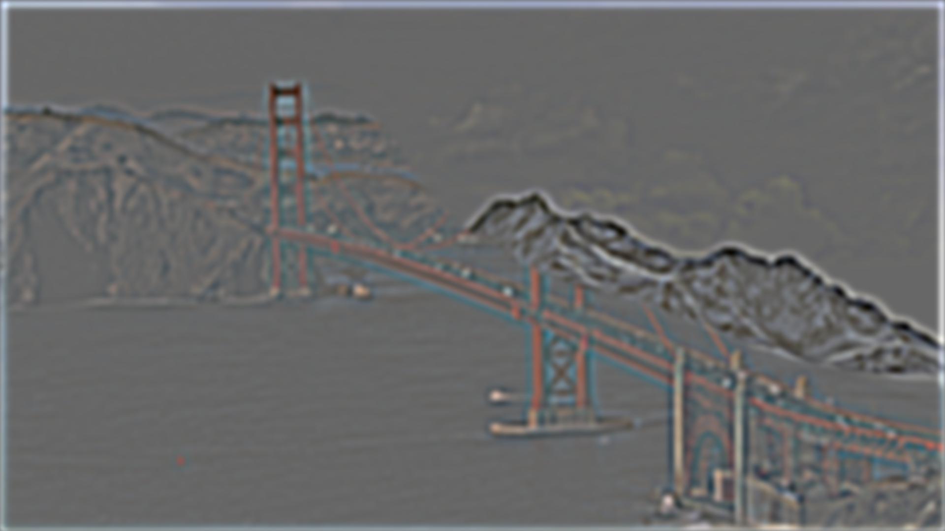
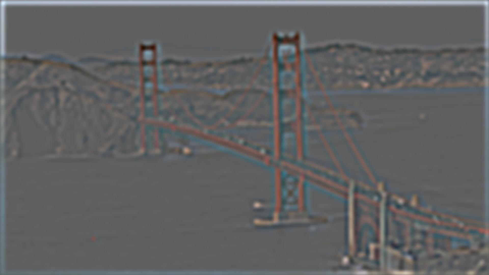
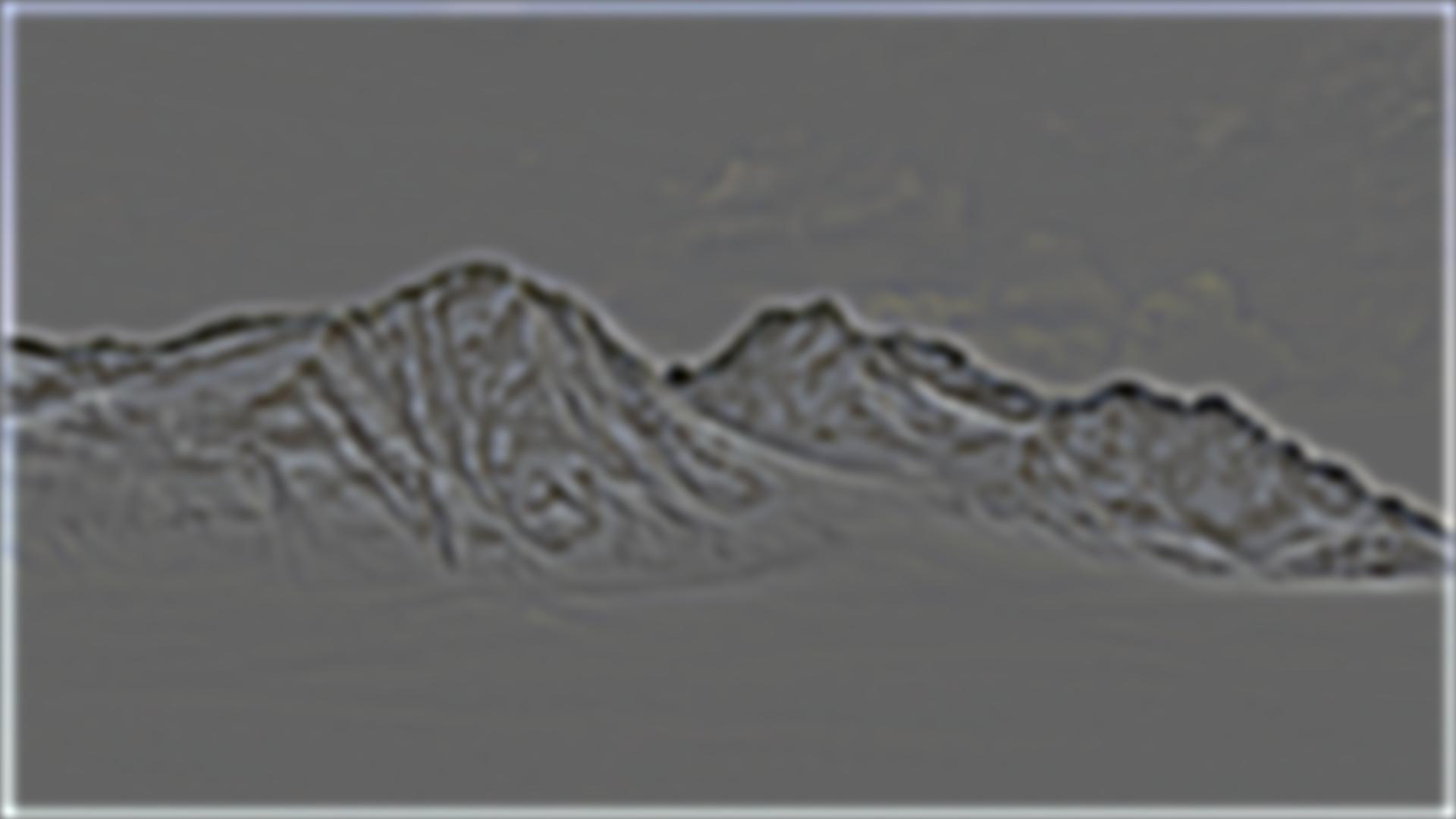
Golden Gate Bridge and Snowy Mountains
 |
 |
 |
 |
 |
 |
 |
 |
 |
 |
 |
 |
 |
 |
 |
 |
 |
 |
 |
 |
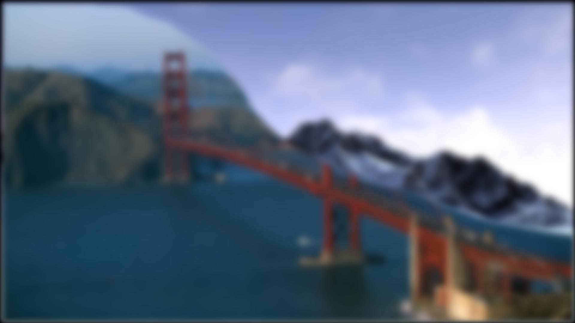 |
This was an amazing project, and I'm blown away by how easy it is to create beautiful blended images by simply summing and aggregating Laplacian stacks! The merged images of the golden gate bridge and the snowy mountains, as well as the blended image of the forest and the beach are breathtakingly beautiful.
FILE = "main.html"

with open(FILE, 'r') as html_file:
    content = html_file.read()

# Get rid off prompts and source code
content = content.replace("div.input_area {
	display: none;","div.input_area {
	display: none;\n\tdisplay: none;")
content = content.replace(".prompt {
	display: none;",".prompt {
	display: none;\n\tdisplay: none;")

f = open(FILE, 'w')
f.write(content)
f.close()