CS 194-26 Project 2: Fun with Filters and Frequencies

Catherine Lu, Fall 2020

Overview

In this project, I worked on various applications of filters in image processing. I used finite difference operators as a simple filter for edge detection with a more complex application in image straightening. I also experimented with Gaussian filters for everything from image sharpening to blending together images and creating Gaussian and Laplacian stacks.

Part 1: Fun with Filters

Part 1.1: Finite Difference Operator

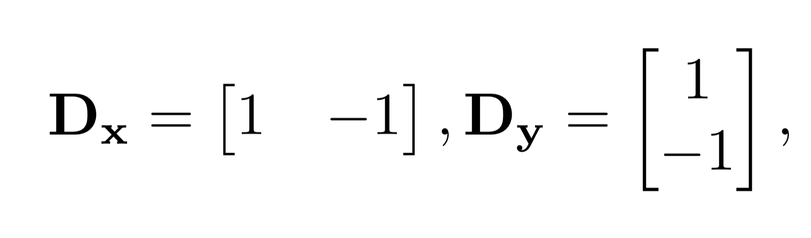
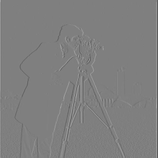
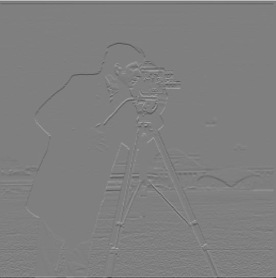
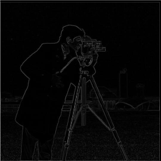
I used the finite difference operator to generate a gradient magnitude image for this photo of a cameraman. Figures 1.1.1 and 1.1.2 show the partial derivatives of the cameraman image in the x and y directions respectively. To compute the gradient magnitude image from these, I took the magnitude of the gradients at each pixel according to the equation below.

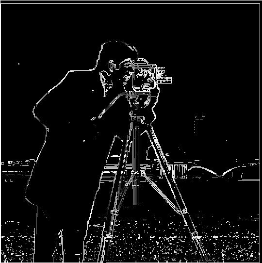
Figure 1.1.1: Partial Derivative in X	Figure 1.1.2: Partial Derivative in Y
Figure 1.1.3: Gradient Magnitude Image	Figure 1.1.4: Binarized Edge Image

Figure 1.1.4 shows the resulting binarized image that is obtained by assigning certain values in the gradient magnitude image to 1 and certain values to 0 according to some threshold.

Part 1.2: Derivative of a Gaussian (DoG) Filter

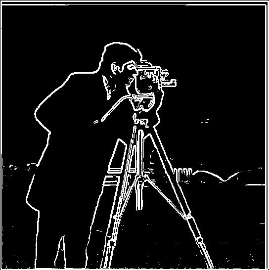
Figure 1.2.1: Binirized Image after Gaussian Blur

In the figure above, we again have the binarized image of the cameraman, but this time after first applying a gaussian blur to the image. This smooths out and gets rid of some of the noise in the image, creating clearer lines for the edges and removing the noise from the field compared to Figure 1.1.4.

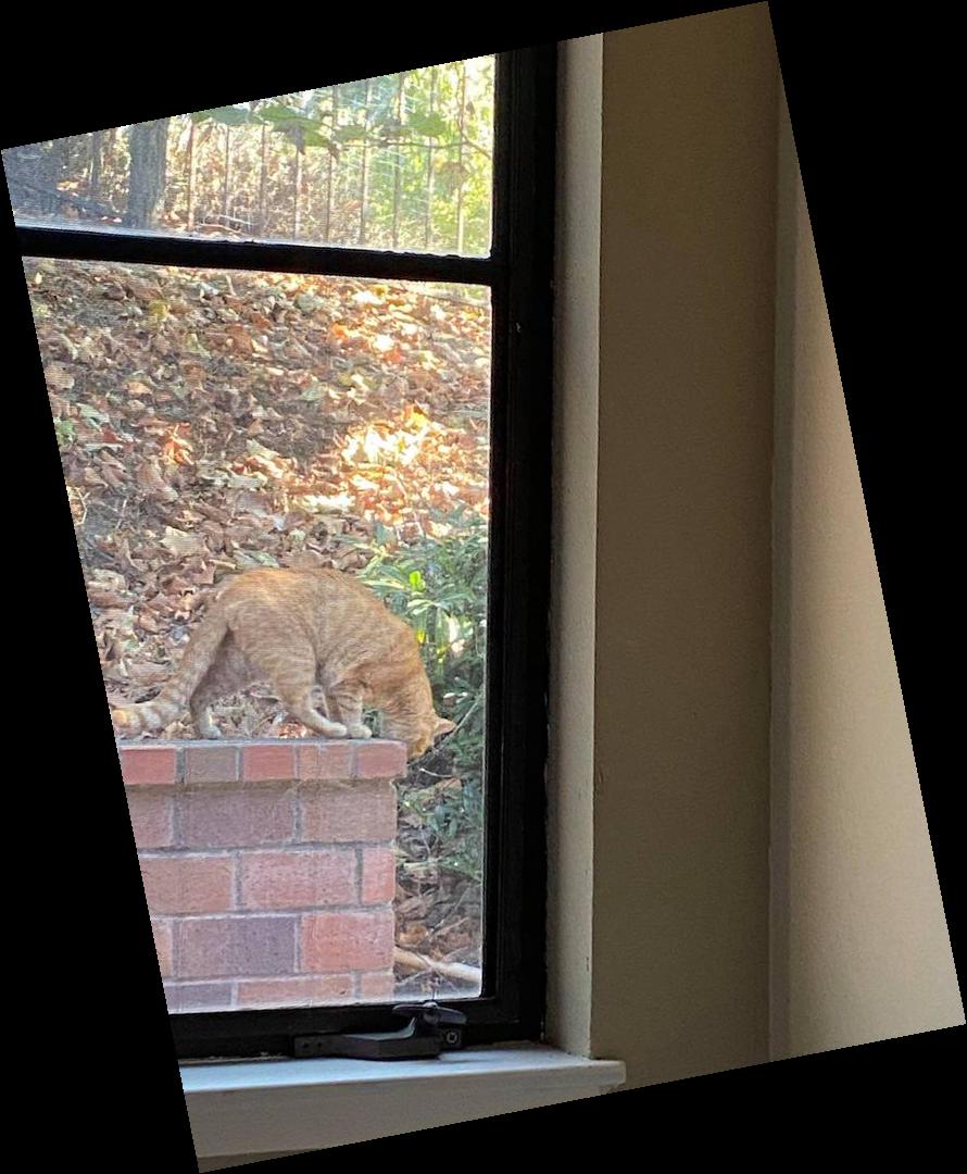
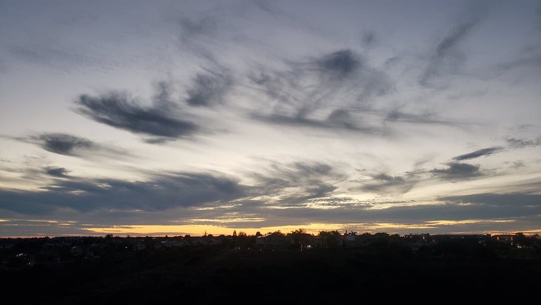
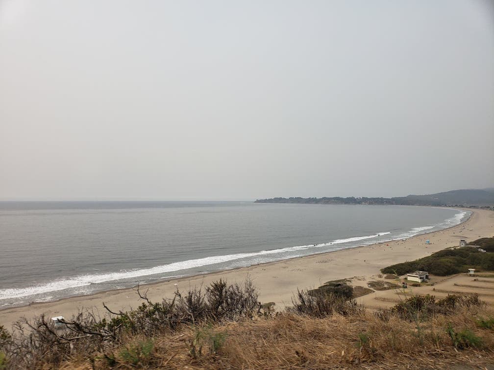
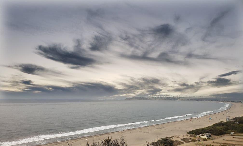
Part 1.3: Image Straightening

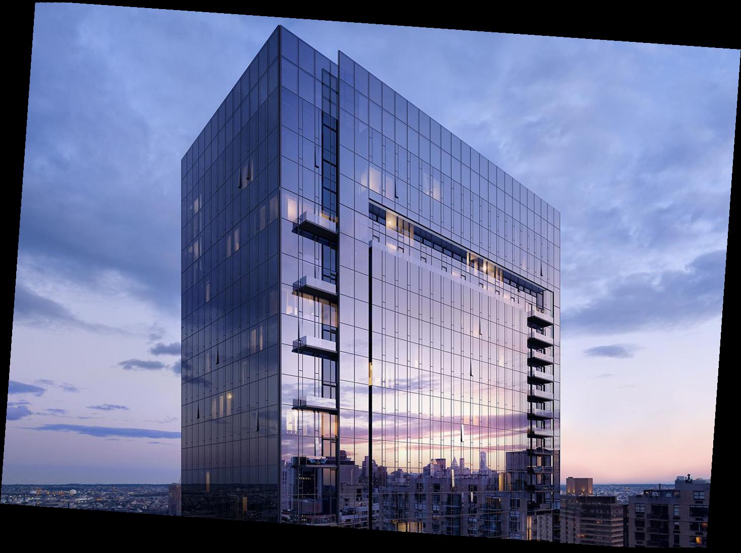
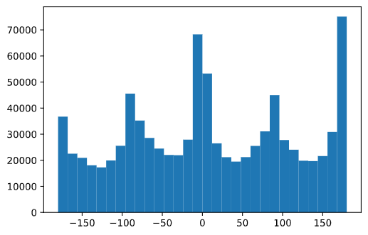
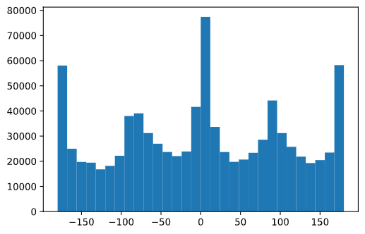
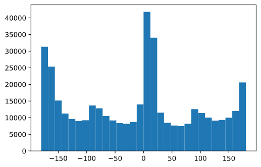
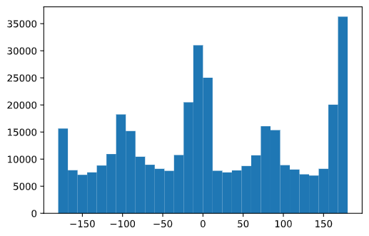
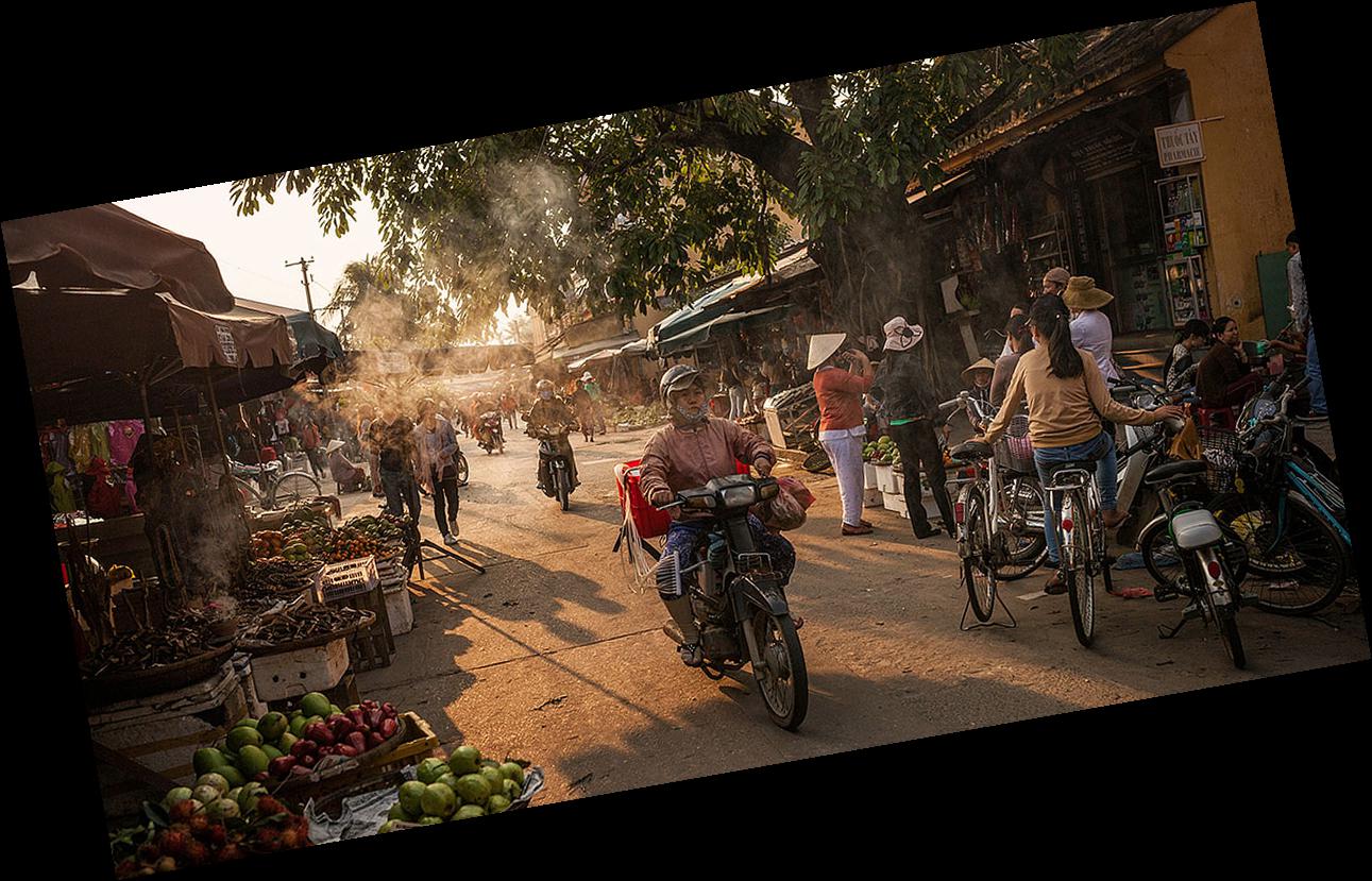
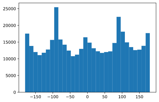
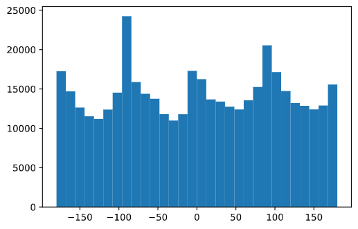
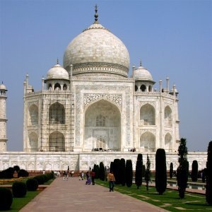
In this apart, I've implemented image straightening based on the preference for vertical and horizontal edges in images. First, I convovled the image with a gaussian filter to get rid of any noise, then computed the partial derivatives in the x and y directions and used these to compute gradient angles. By repeating this process for a range of possible rotation angles, I used the angle with the highest amount of horizontal and vertical edges to obtain the straighted image. The images below display some examples of aligned images and the gradient angle histograms.

Facade Image
Facade Original	Straightened Facade
Gradient Angles for Original Facade Image	Gradient Angles for Straightened Facade Image

Glass Building Image
Glass Building Original	Straightened Glass Building
Gradient Angles for Original Glass Building Image	Gradient Angles for Straightened Glass Building Image

Cat Image
Cat Original	Straightened Cat
Gradient Angles for Original Cat Image	Gradient Angles for Straightened Cat Image

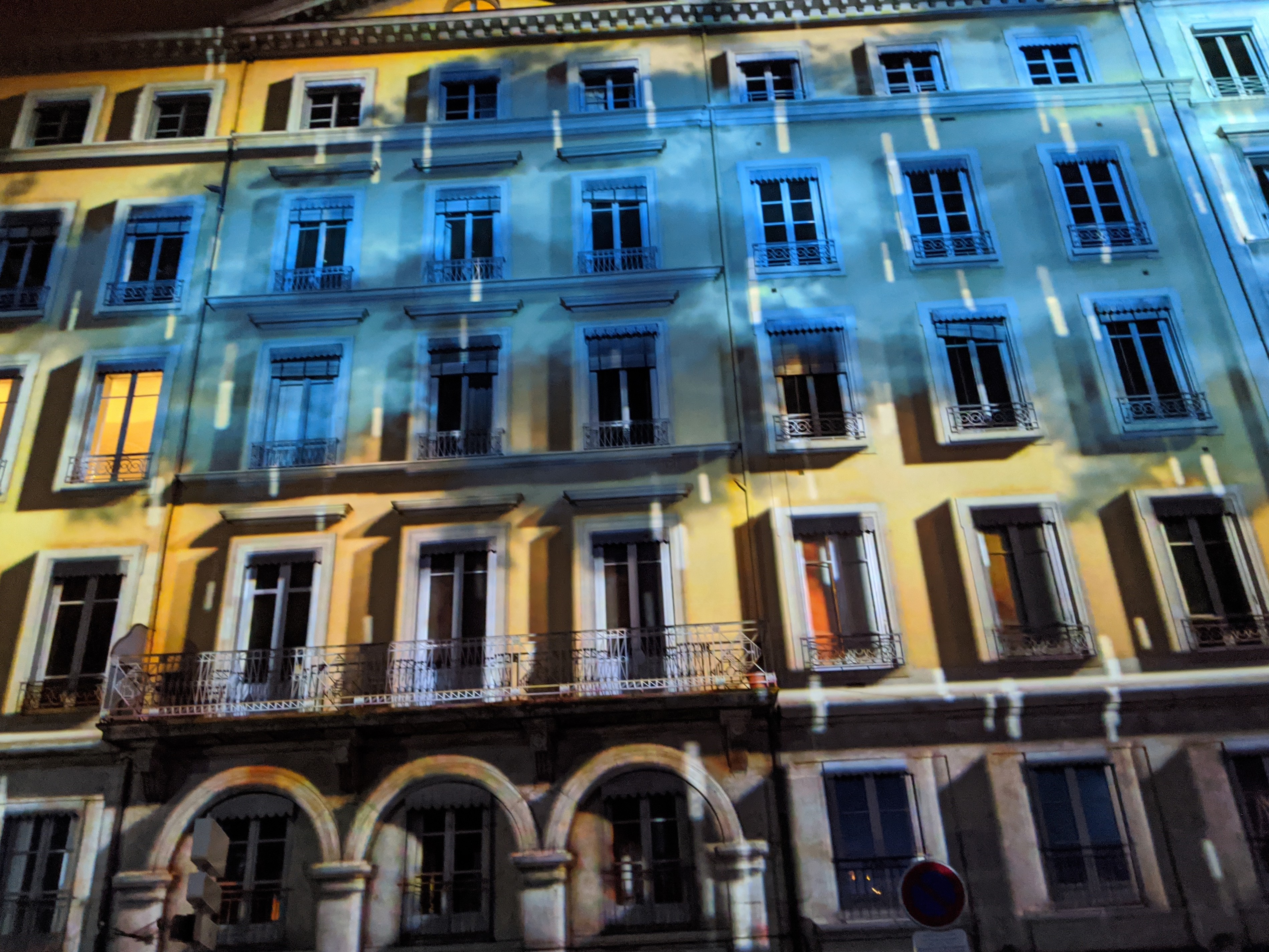
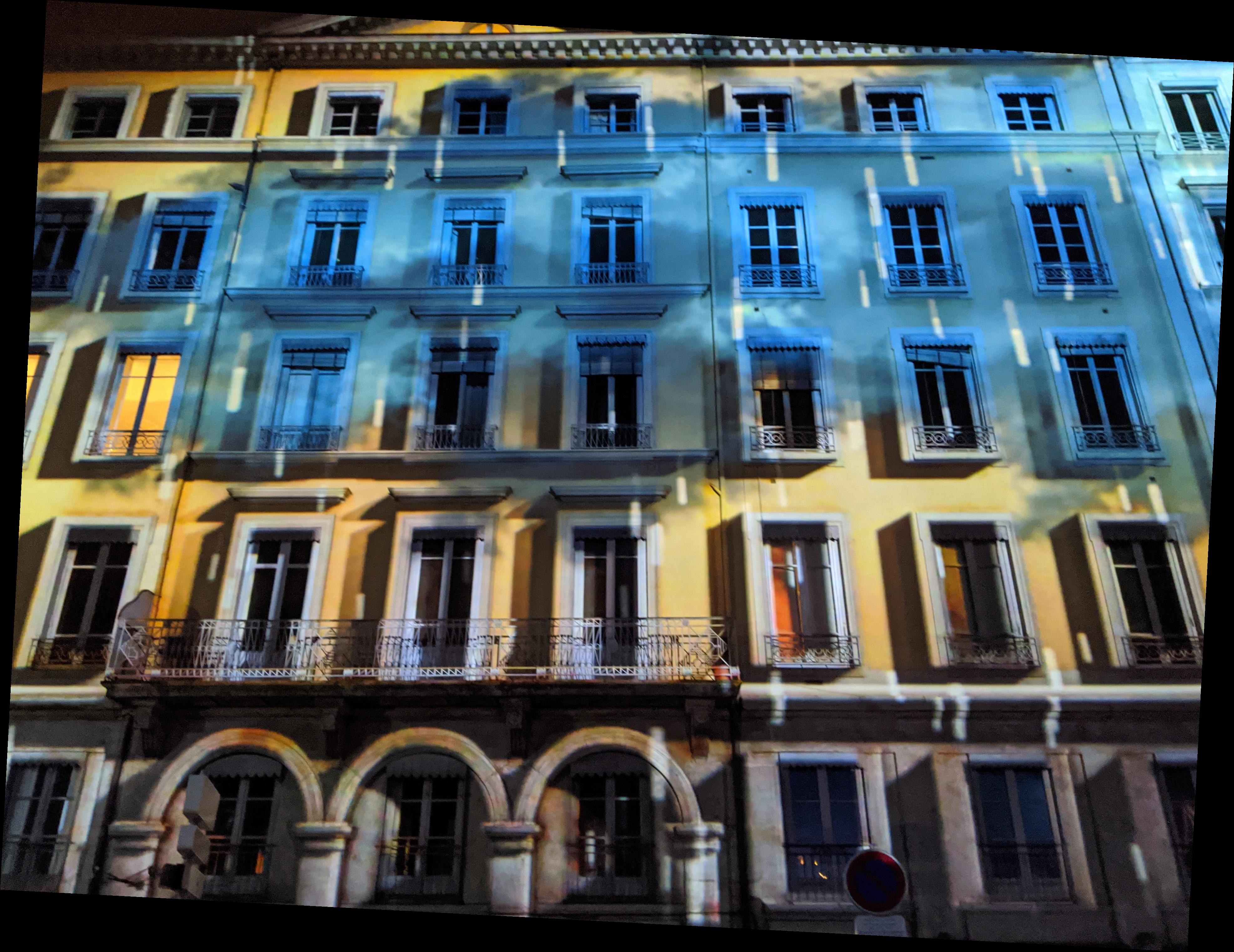
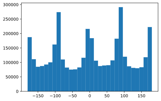
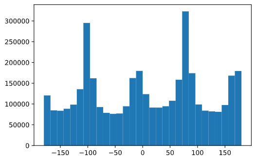
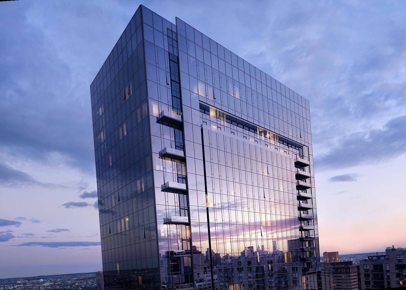
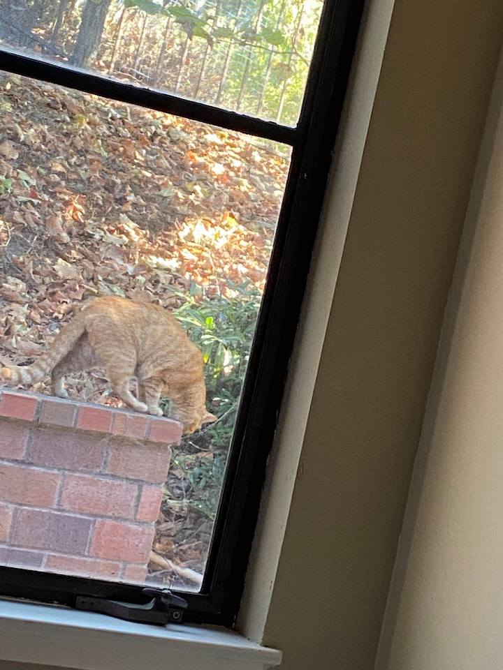
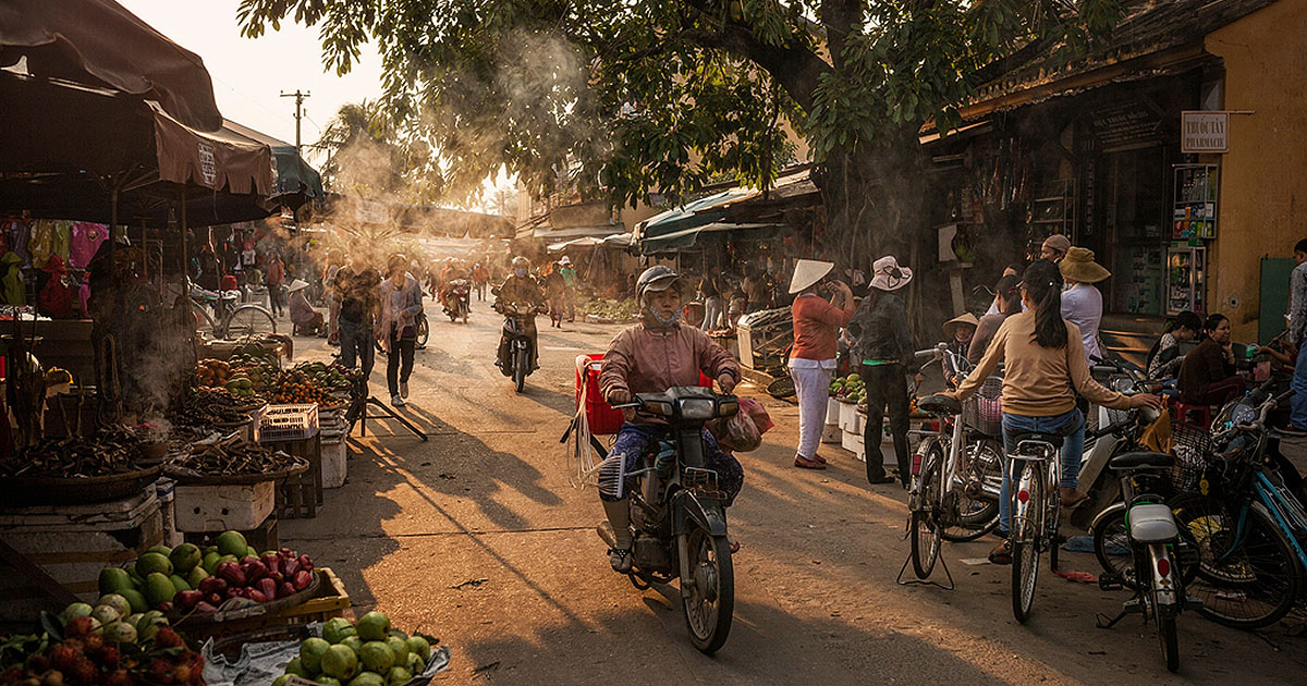
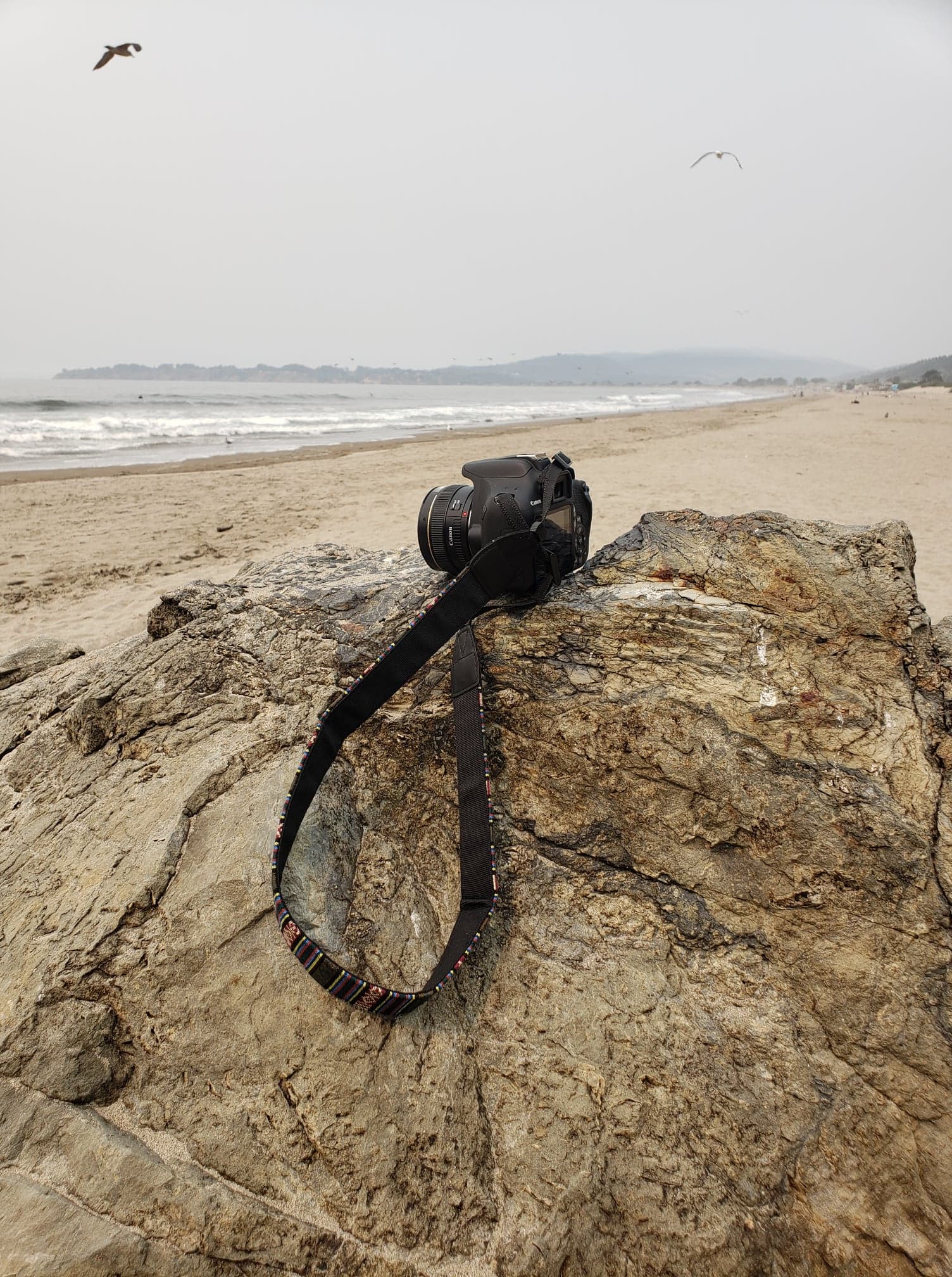
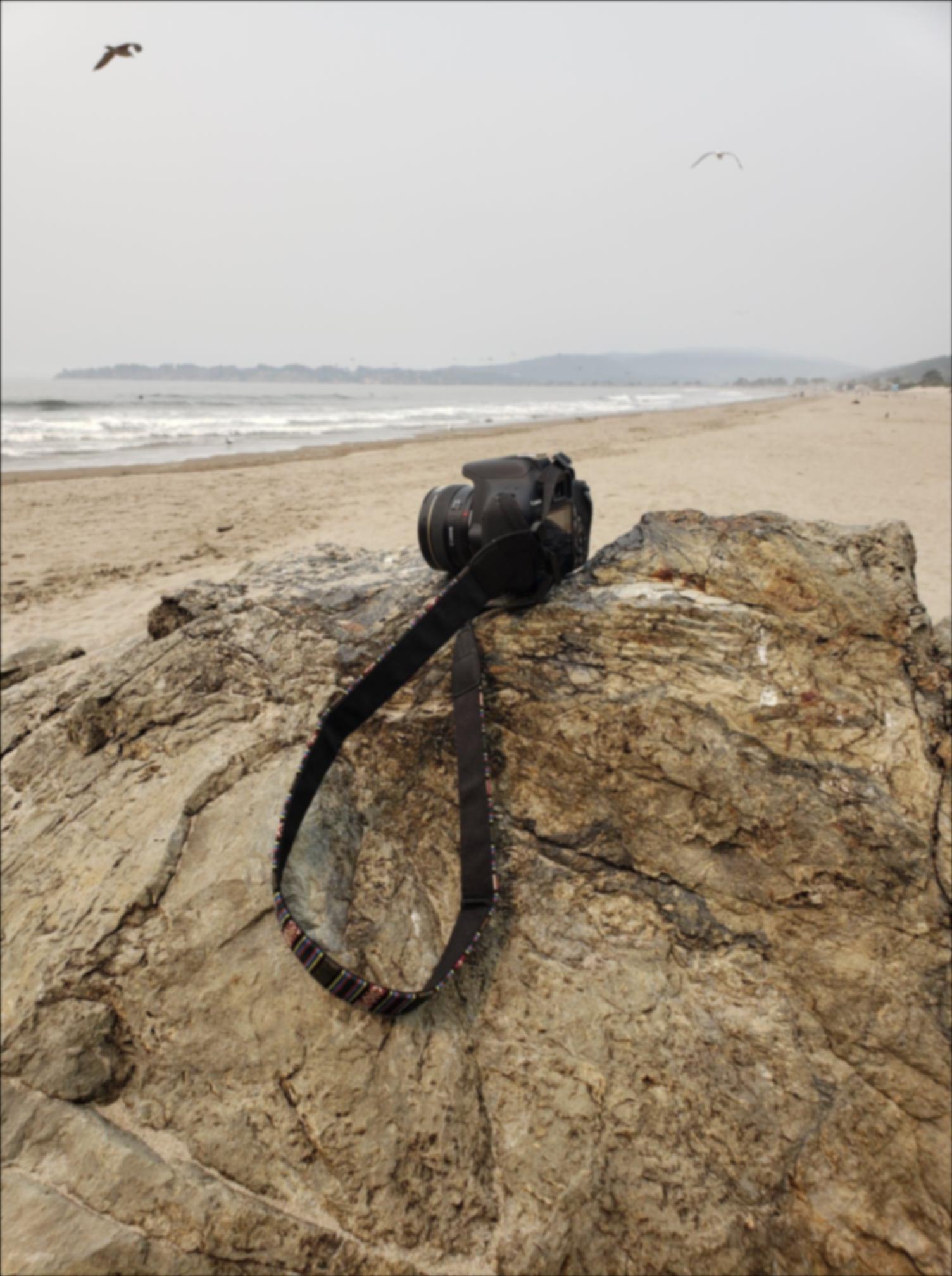
While this method may work well for many images, it also has some problems. In the example below, there are no clear horizontal or vertical edges as there are many objects in the image and the perspective of the image makes it so that any originally straight edges should now be slanted in an edge-straighted image.

Failure Case: Street Image
Street Original	Rotated Street
Gradient Angles for Original Street Image	Gradient Angles for Rotated Street Image

Part 2: Fun with Frequencies!

Part 2.1: Image "Sharpening"

Figure 2.1.1: taj.jpg - Original	Figure 2.1.2: taj.jpg - Sharpened
Figure 2.1.3: cat.jpg - Original	Figure 2.1.4: cat.jpg - Sharpened

The images in the figures above have been "sharpened" by using a Gaussian kernel to blur the image, then subtracting the blurred image from the original image to obtain only the high frequencies, and adding the high frequencies back in. These operations can be combined into a single convolution using the unsharp mask filter.

Figure 2.1.5: camera_rock.jpg - Original

Figure 2.1.6: camera_rock.jpg - Blurred

Figure 2.1.7: camera_rock.jpg - Sharpened

However, this process does not actually sharpen the image because there is no new information being added in. It only magnifies the existing high frequencies in the image. This is illustrated by the images above where the image is blurred and then the blurred image is sharpened. This does not produce the original image but rather a version of the blurred image with "sharper" edges.

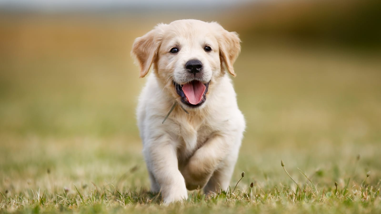
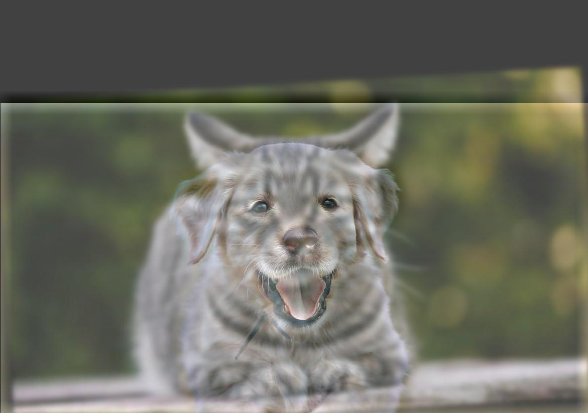
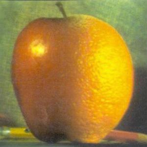
Part 2.2: Hybrid Images

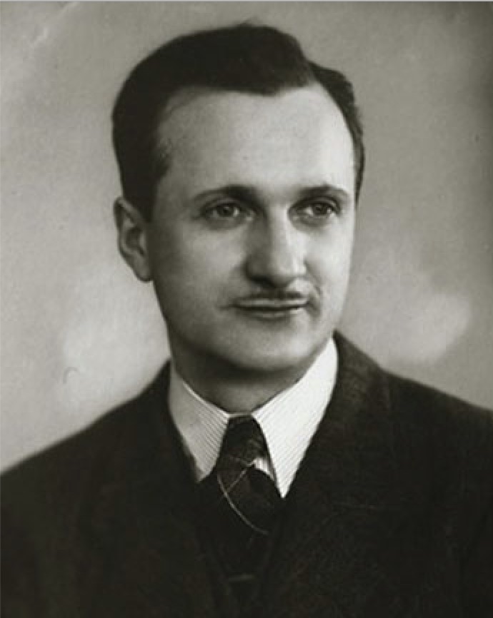
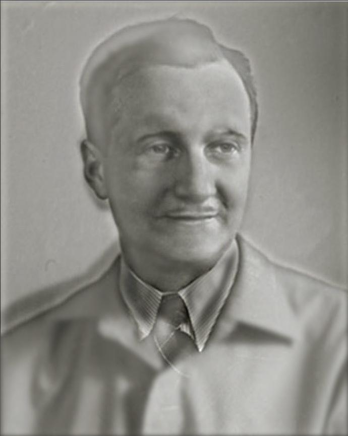
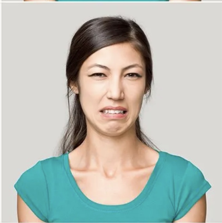
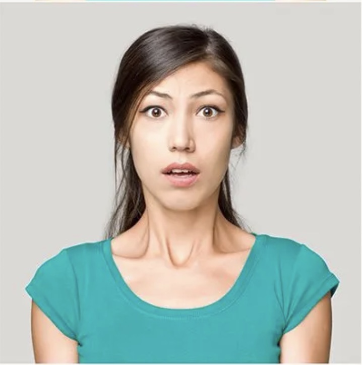
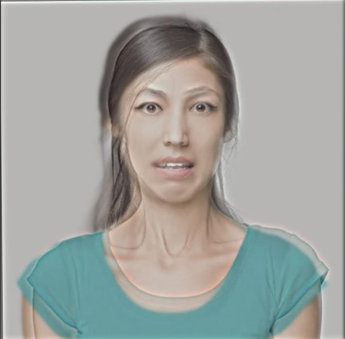
Hybrid images are images that have a different interpretation at different viewing distances. The hybrid images here are generated by taking the high frequencies of one image and overlaying them on the low frequencies of a different image. The resulting image will look like the high frequency image at close distances and look like the low frequency image at far distances. Below are some examples of such hybrid images that show change in age and change in expression at different distances.

Figure 2.2.1: Young Man

Figure 2.2.2: Old Man

Figure 2.2.3: Young/Old Hybrid

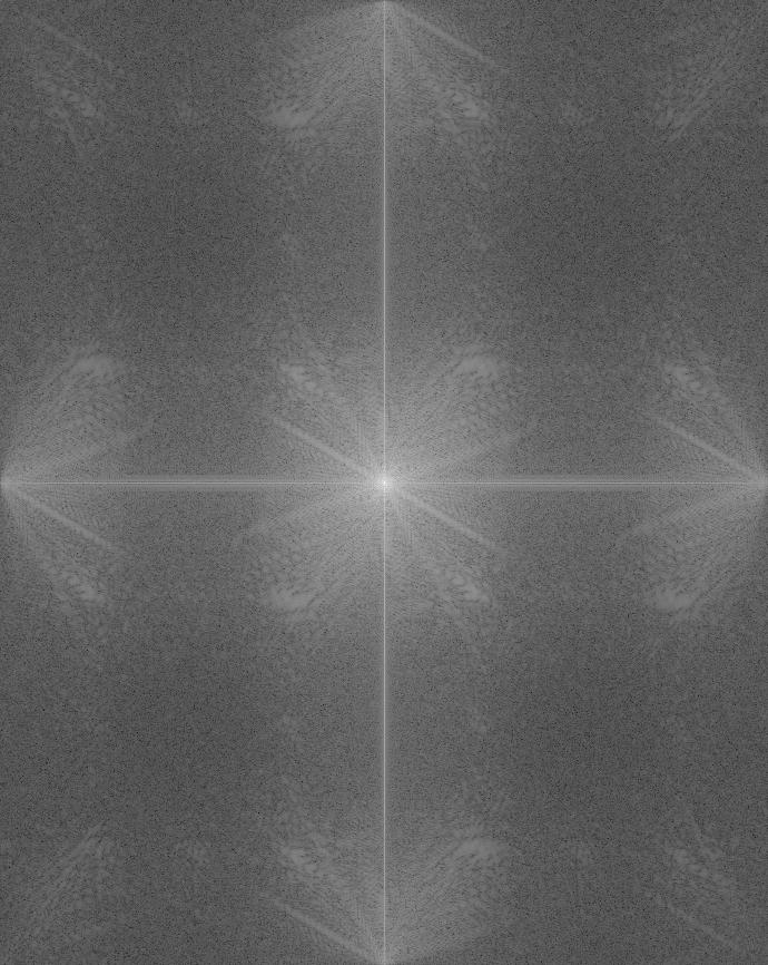
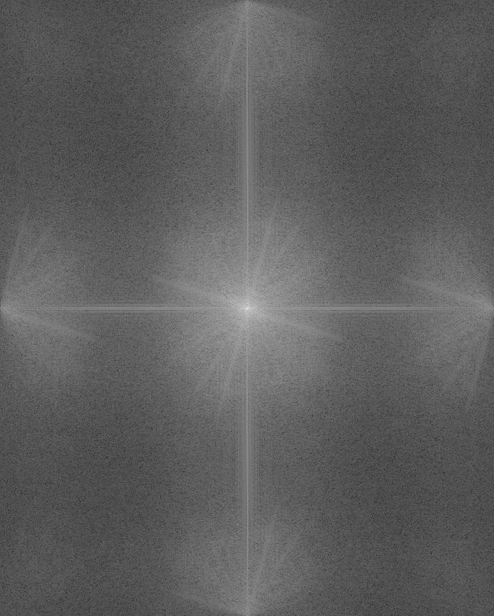
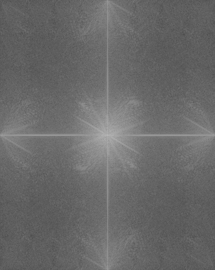
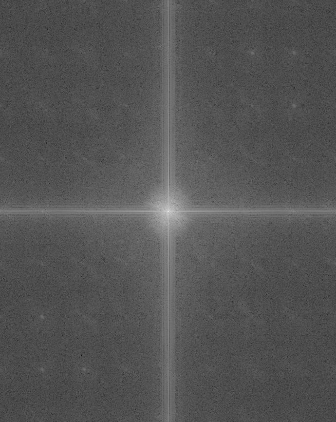
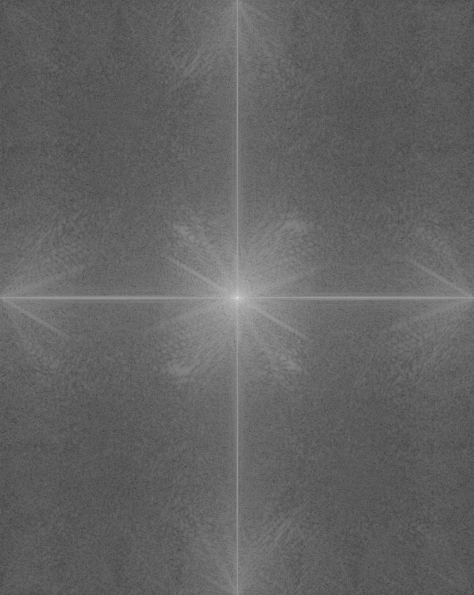
The table of images below show the various stages of Young/Old Man hybrid image in the frequency domain.

FFT for Young/Old Man Hybrid Process
Young Man FFT	Old Man FFT	Young High Frequencies	Old Low Frequencies	Young/Old Hybrid FFT

Figure 2.2.4: Disgust Expression

Figure 2.2.5: Surprise Expression

Figure 2.2.6: Disgust/Surprise Hybrid

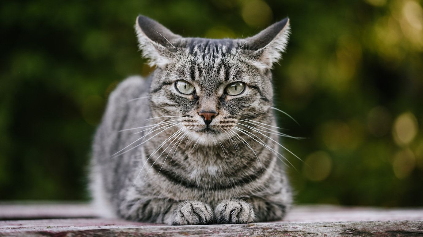
The images below show a failure case in generating hybrid images. This example fails because the cat and the dog have very different face shape, so even after aligning the eyes, the rest of the features are nowhere close to matching up. This creates a very messy result.

Figure 2.2.7: Cat

Figure 2.2.8: Dog

Figure 2.2.9: Cat/Dog Hybrid

Part 2.3: Gaussian and Laplacian Pyramids

The first table of images shows a Gaussian stack which is created by blurring successive images with a gaussian filter. The second table of images shows a Laplacian stack which is created by taking the difference between successive images in the Gaussian stack and then appending the last image from the Gaussian image to the bottom of the stack. Thus, the Gaussian stack just contains the original image directly in the stack while for the Laplacian stack, the original image can be obtained by summing together all the images in the stack.

Using the Gaussian and Laplacian stacks, we can also break down the construction of the hybrid images. In the hybrid of the young man and old man the Gaussian stack shows us the old man clearly because we are blurring the image to show only the lower frequencies at each stage of the stack. The Laplacian stack on the other hand shows us the young man clearly initially because it extracts the high frequencies of the image.

Part 2.4: Multiresolution Blending

In this part of the project, I performed multiresolution by creating laplacian stacks for the two images I was blending together and creating a gaussian stack for a mask of each image. Then I summed the masked images at each level of the stack to create the resulting blending image.

Apple

Orange

Oraple

Sunset

Beach

Beach with sunset

Night Sky

Mooncake

Mooncake as Moon