Fun with Filters and Frequencies!
Part 1: Fun with Filters
Part 1.1: Finite Difference Operator
In this part we start off by computing the gradient of an image. First, we get a differene operator:
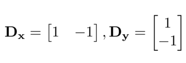
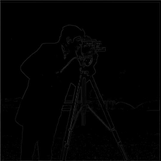
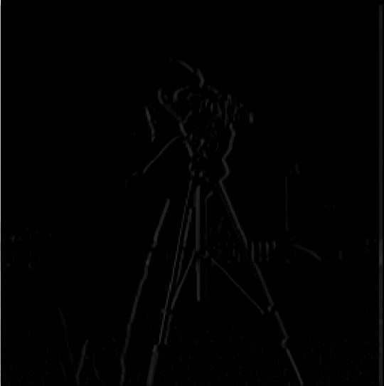
after that, we convolute the operator over the gray scale image. In order to find the gradient magnitude, we take the square root of sum of the squared partial derivatives. After that, we binarize the gradient magnitude with a self-defining threshold.
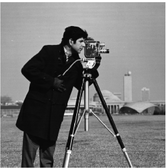
original camerman
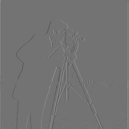
camerman x-direction derivative
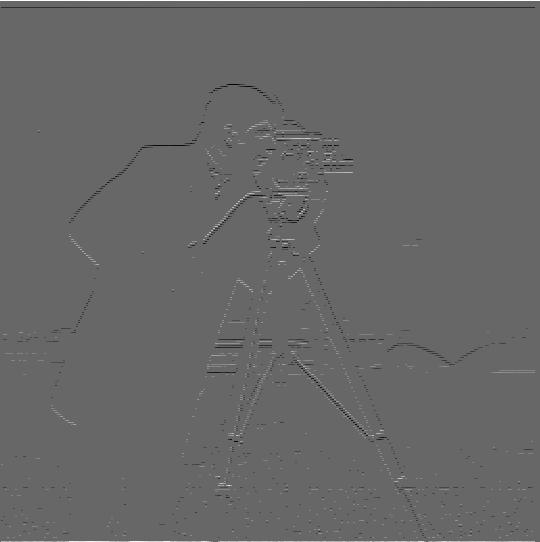
camerman y-direction derivative
cameraman gradient image
Part 1.2: Derivative of Gaussian (DoG) Filter
In this part, we do a very similar thing as we did in 1.1. What we are doing here is a Gaussian filter. As we can see, there is still some noise in the images. We want to reduce the noise of the edge images by first blurring our image by running it through a gaussian filter, and we do the same operations as before. After that, we can see that the final image becomes less noisy. Also, We can further improve this process doing one convolution instead of two by using the derivative of Gaussian filters, and the results should be the same.
camerman image with Gaussian and dx
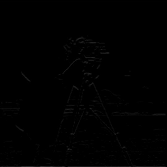
camerman image with Gaussian and dy
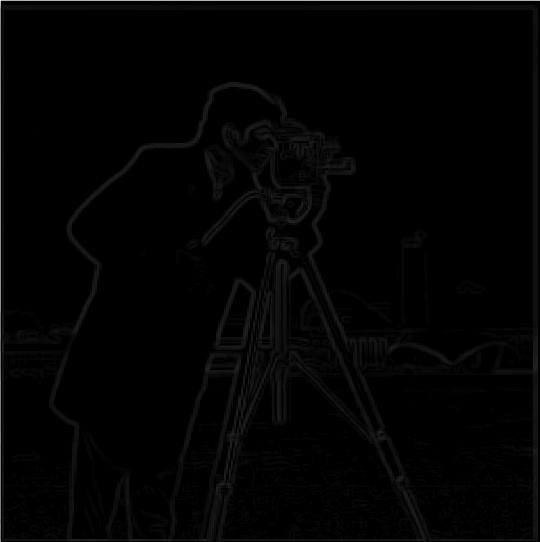
camerman image with DoG
Part 1.3: Image Straightening
This section is more mathematically heavy. It is all about image straightening algorithm. The algorithm is: Firstly, rotate the image by some angle "ang". Then, compute the gradient angle of all the edges in the rotated image by using arctan function. After that, we get a histogram of these angles from above operations. Finally, return the image with the highest number of gradient angles equal to -180 degree, -90 degree, 0, 90 degree, or 180 degree, which are the "straightest" ones.
Facade
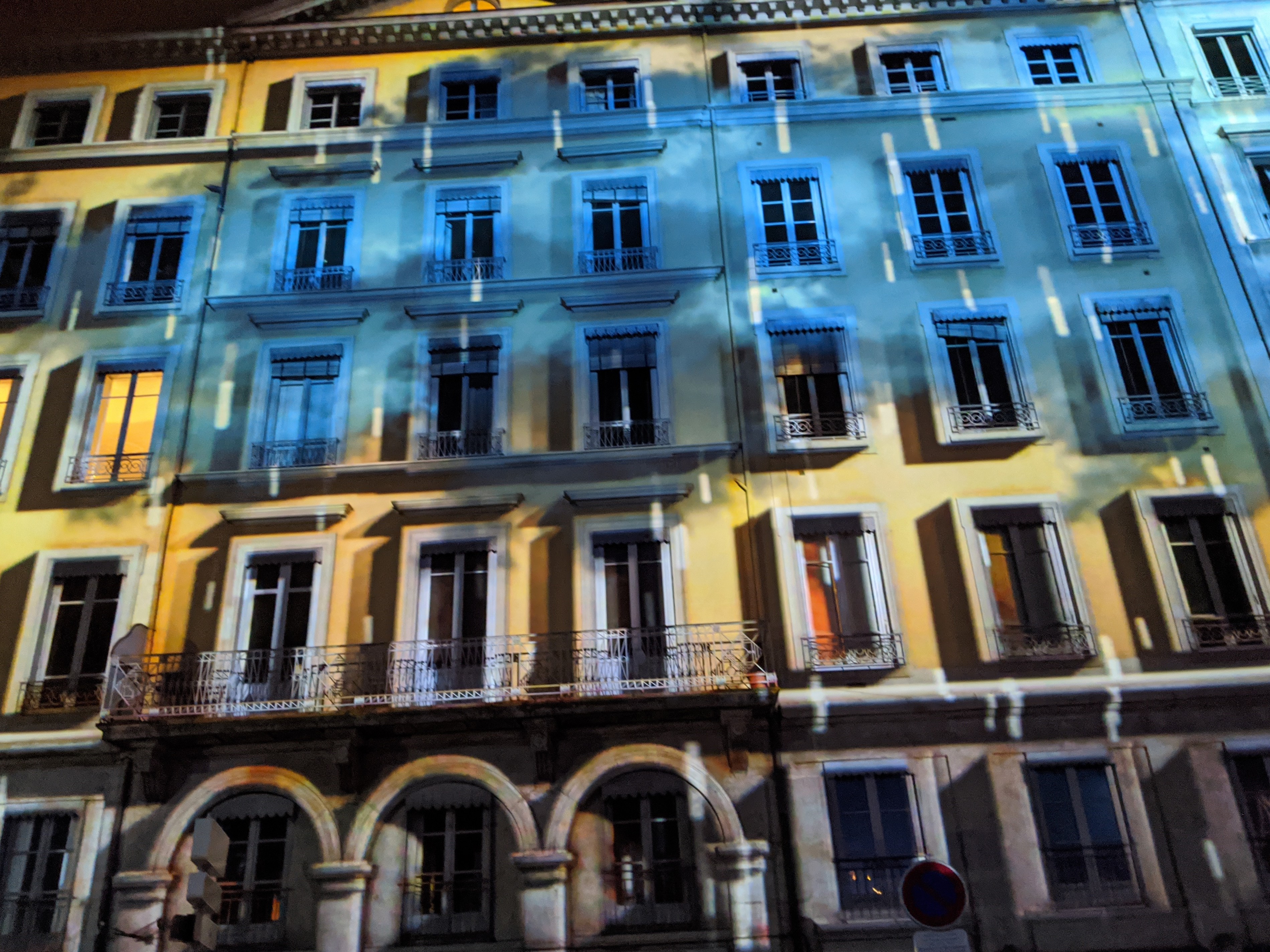
Facade
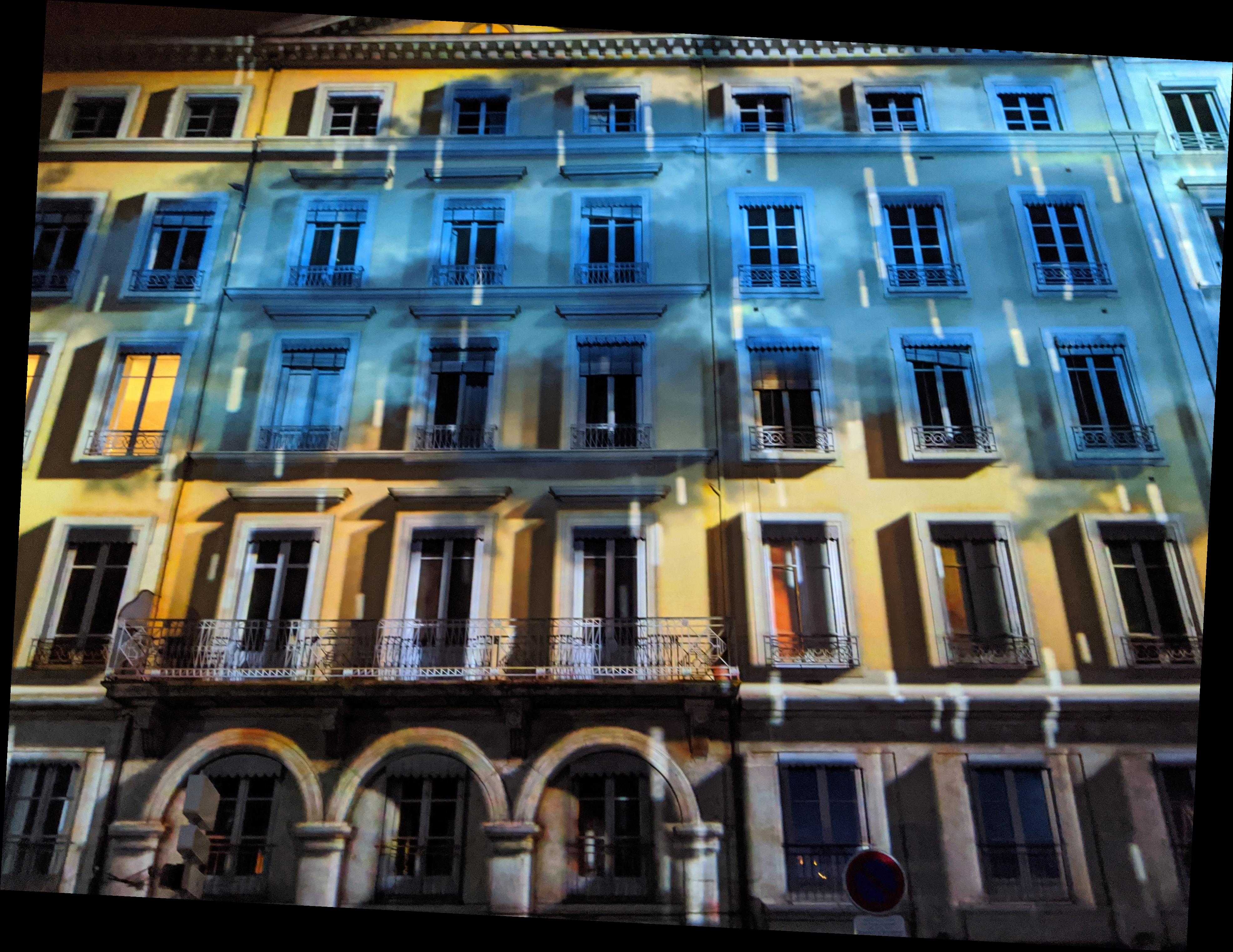
Facade after rotaion -3
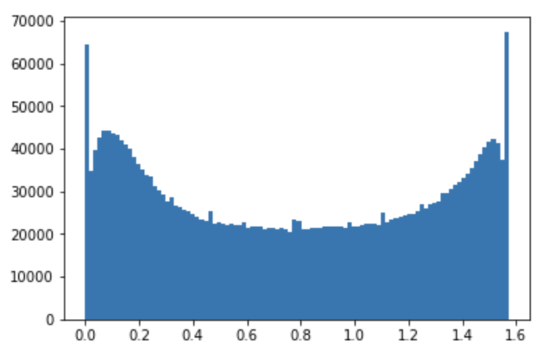
Facade Histgram (Unrotated)
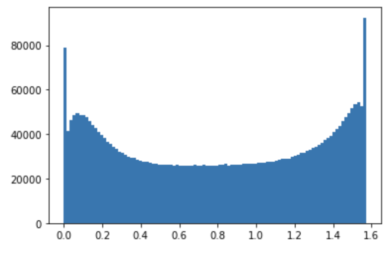
Facade Histgram (Rotated -3)
Pisa Tower
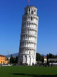
Pisa
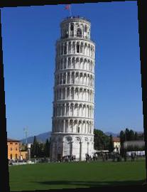
Pisa after rotation +7
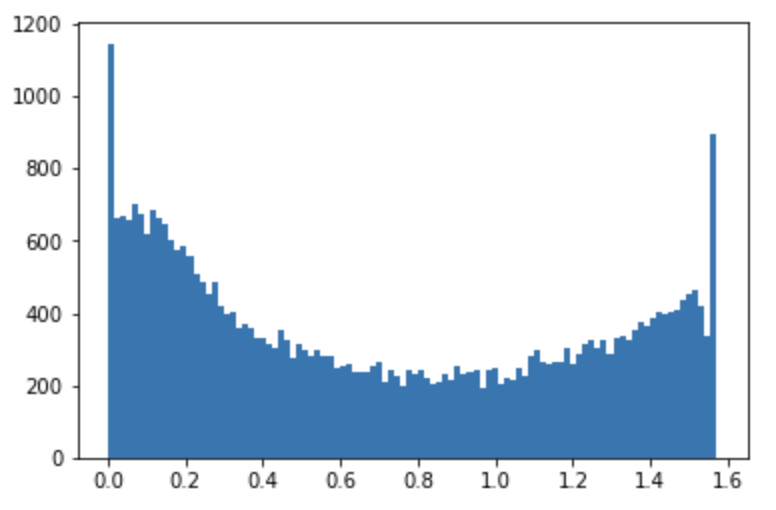
Pisa Histgram (Unrotated)
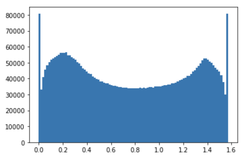
Pisa Histgram (Rotated +7)
KFC

KFC
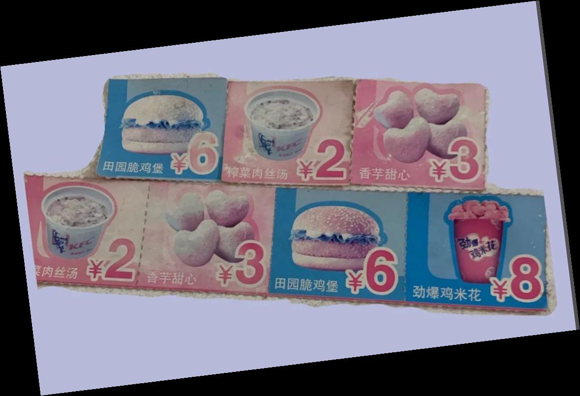
KFC after rotation +7
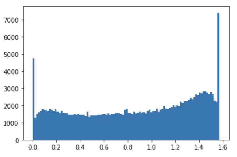
KFC Histgram (Unrotated)
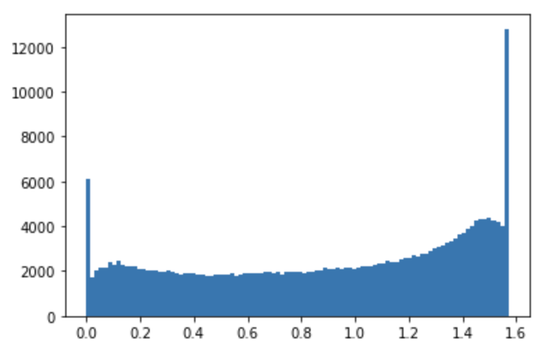
KFC Histgram (Rotated +7)
Failure Case: Kabab
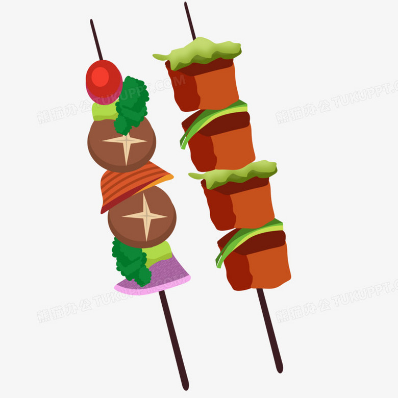
Kabab
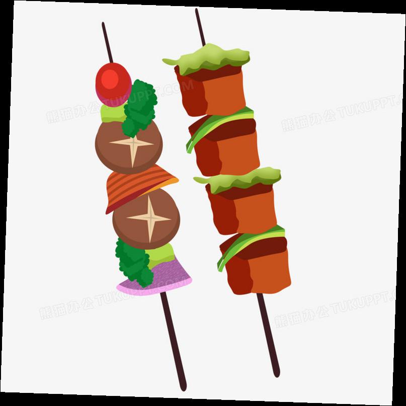
Kabab after rotation-2
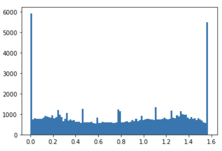
Kabab Histgram (Unrotated)
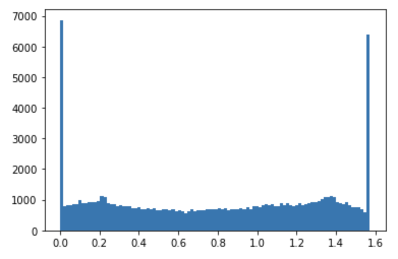
Kabab Histgram (Rotated -2)
Part 2: Fun with Frequencies
Part 2.1: Image "Sharpening"
In this part, we did image sharpening, which is done by adding higher frequencies from an image to the image itself. In order to get the high frequencies, we subtract the blurred image from itself and convolve the image with a Gaussian from the original picture. After that, we add these high frequencies to the original image. Notice that we are not sharpening an image by actually getting a higher resolution, so it is more like a "fake" one.
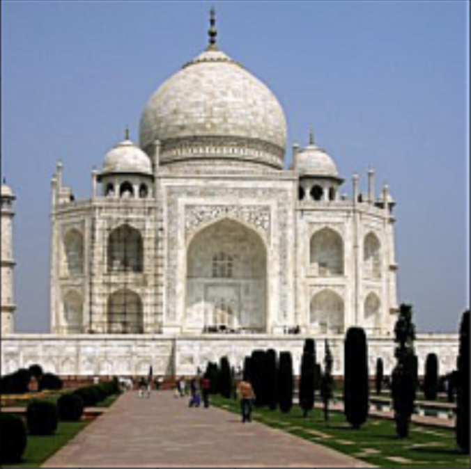
blur taj
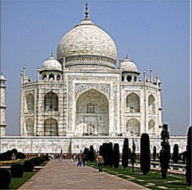
Sharpened taj

Blur cat
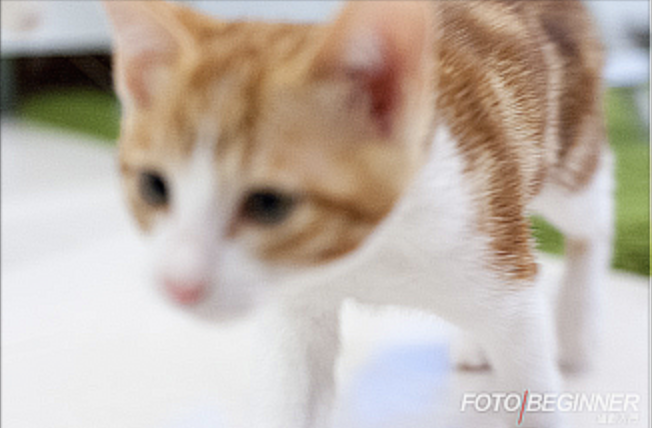
Sharp cat

Sushi

blur Sushi
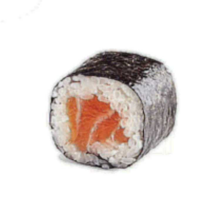
Resharpened blur sushi
Part 2.2: Hybrid Image
We are doing hybrid imaging in this part. First, we align two images. After that, we take the low frequency from image one and take the high frenquency from image two. The basic idea is that high frequency tends to dominate perception when it is available, but, at a distance, only the low frequency (smooth) part of the signal can be seen. By blending the high frequency portion of one image with the low-frequency portion of another, you get a hybrid image that leads to different interpretations at different distances.
Fourier of Derek Image
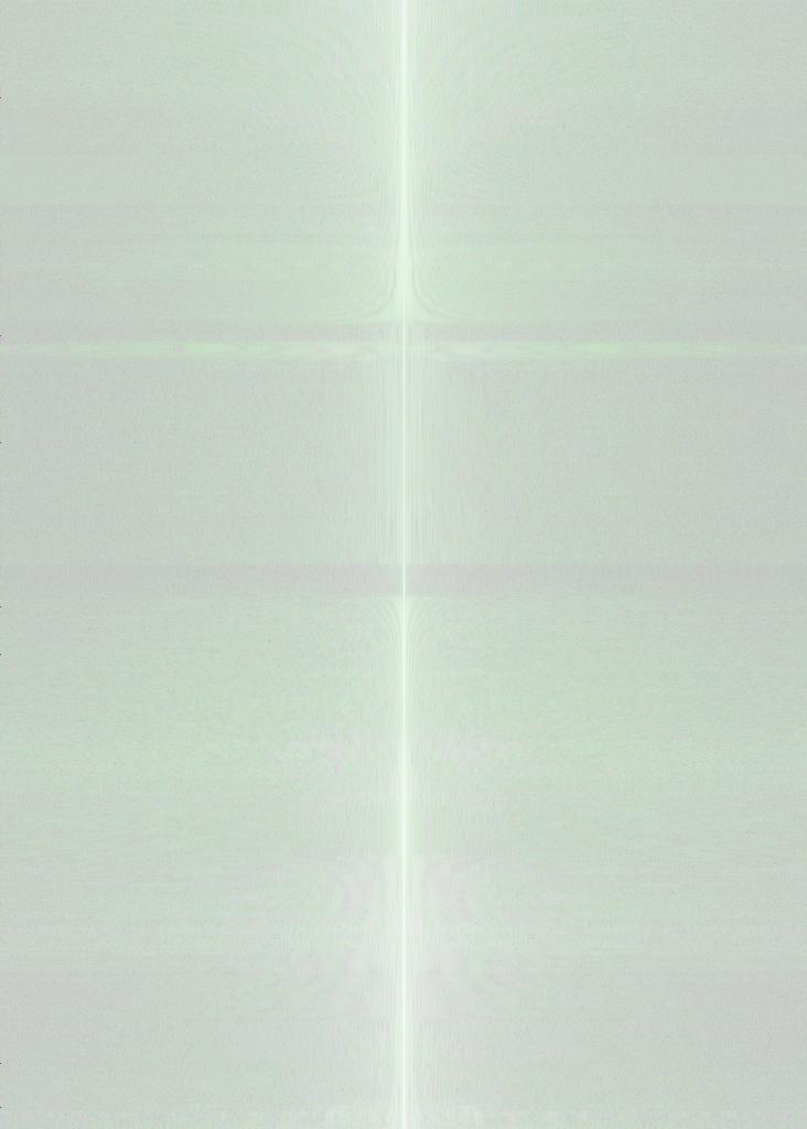
Fourier of Nutmeg Picture
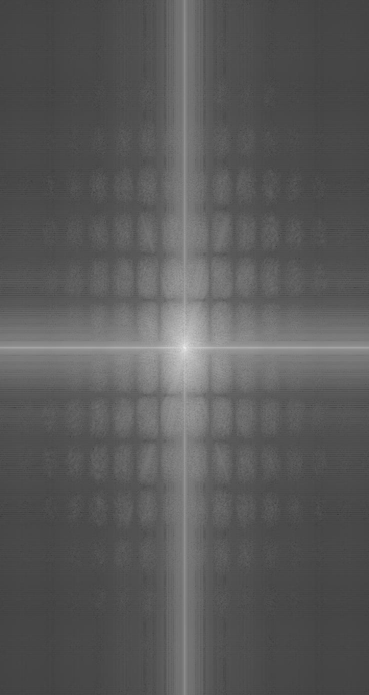
Fourier of Low Frequency Image
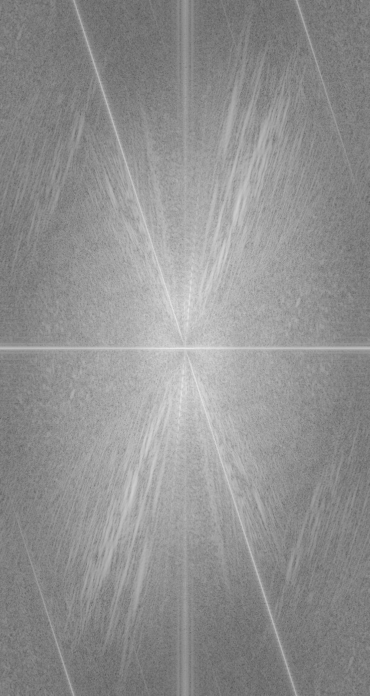
Fourier of High Frequency Image
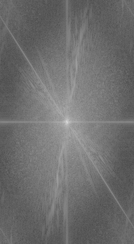
Fourier of Hybrid Image
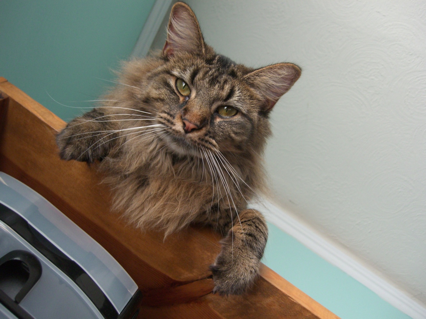
Cat
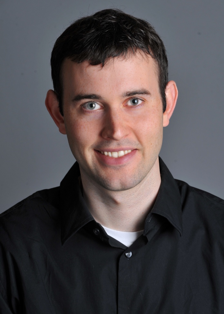
Derek
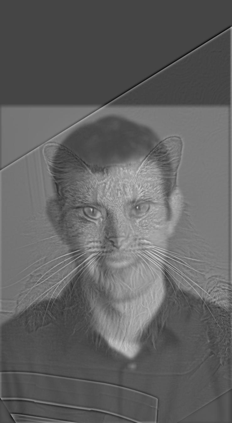
Cat x Derek
The seal x monalisa case is failed, since the cartoon seal is too dominating in the hybrid image. However, the trump x biden case is very successful.
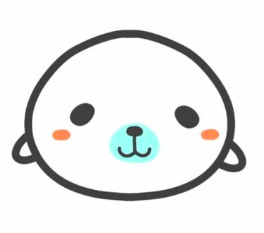
Cartoon Seal
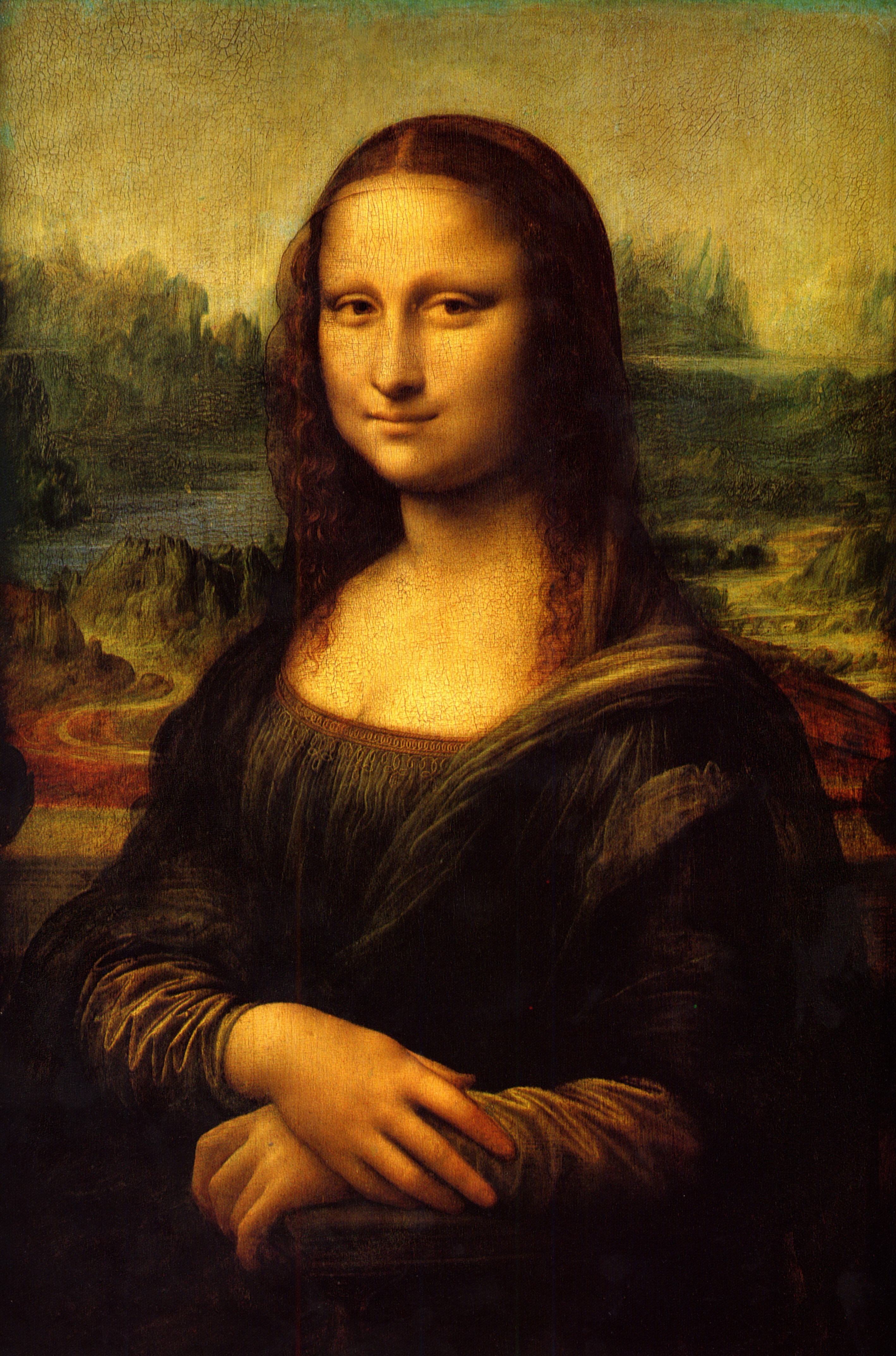
Monalisa
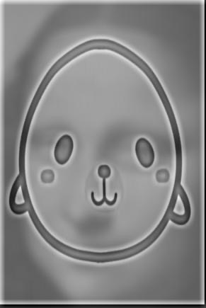
Cartoon Seal x Monalisa (Failed)
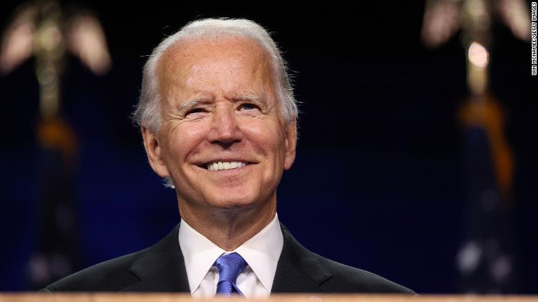
Biden
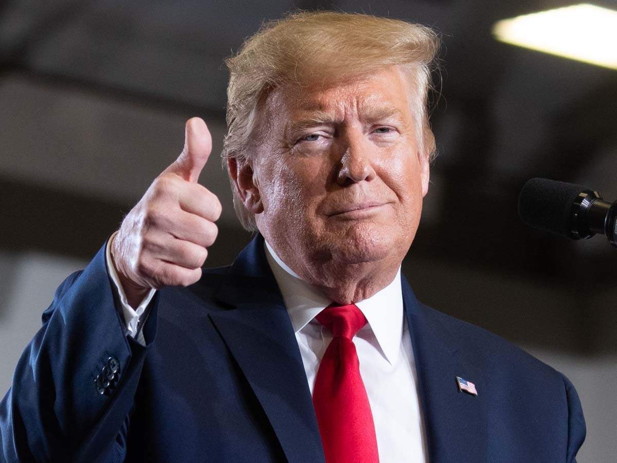
Trump
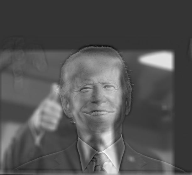
Trump x Biden
Part 2.3: Gaussian and Laplacian Stacks
In this part we implement the the Gaussian stack and the Laplacian stack, which are similar to pyramids except the fact that the images are not downsampled. The Gaussian stack is from applyng Gaussian filter to the same image several times, and put them together in a stack. Laplacian stack is from taking the difference between two images next to each other in the Gaussian Stack
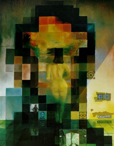
Gaussian Stack of Lincoin and Gala
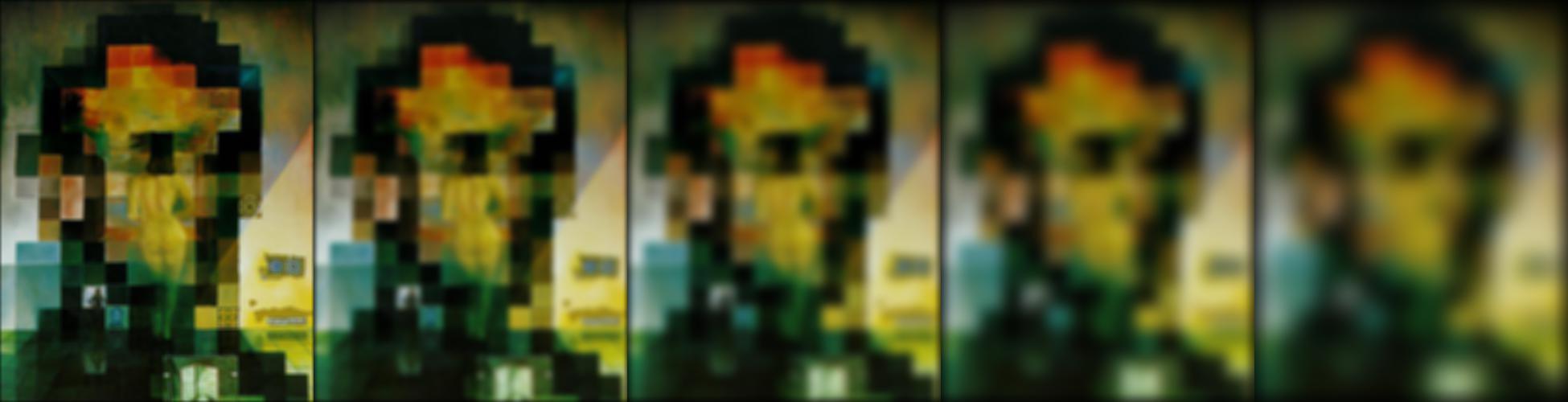
Gaussian Stack of Lincoin and Gala
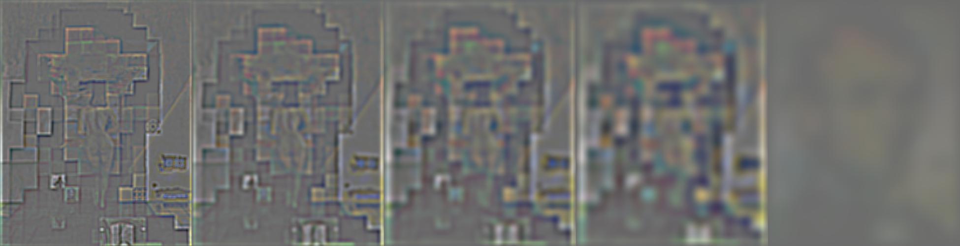
Laplacian Stack of Lincoin and Gala
Part 2.4: Multiresolution Blending
In the last part, we are trying to blend two images into one image by using a mask. At the same time, in order to truly "blend" it, we want to make the blended image as seamless as possible. The technique is all about an algorithm: We start with two images, A and B, and a mask. To make the blended image more seamless, we do the following: 1. Build Laplacian L_A and L_B for image A and image B. 2. Build Gaussian GM for the mask M. 3. Form a combined pyramid L_C (from L_A and L_B), use the nodes of GM as weights: L_C[l] = GM[l] * L_A[l] + (1 - GM[l]) * L_B[l], with l refers to layer. Finally, we will obtain the combined image IMG by summing all levels of L_C.
AppleOrange Mask
My Seal Mask

Apple

Orange
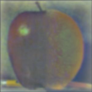
Oraple
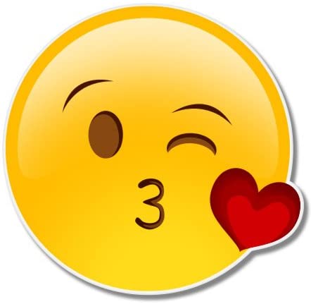
Emoji
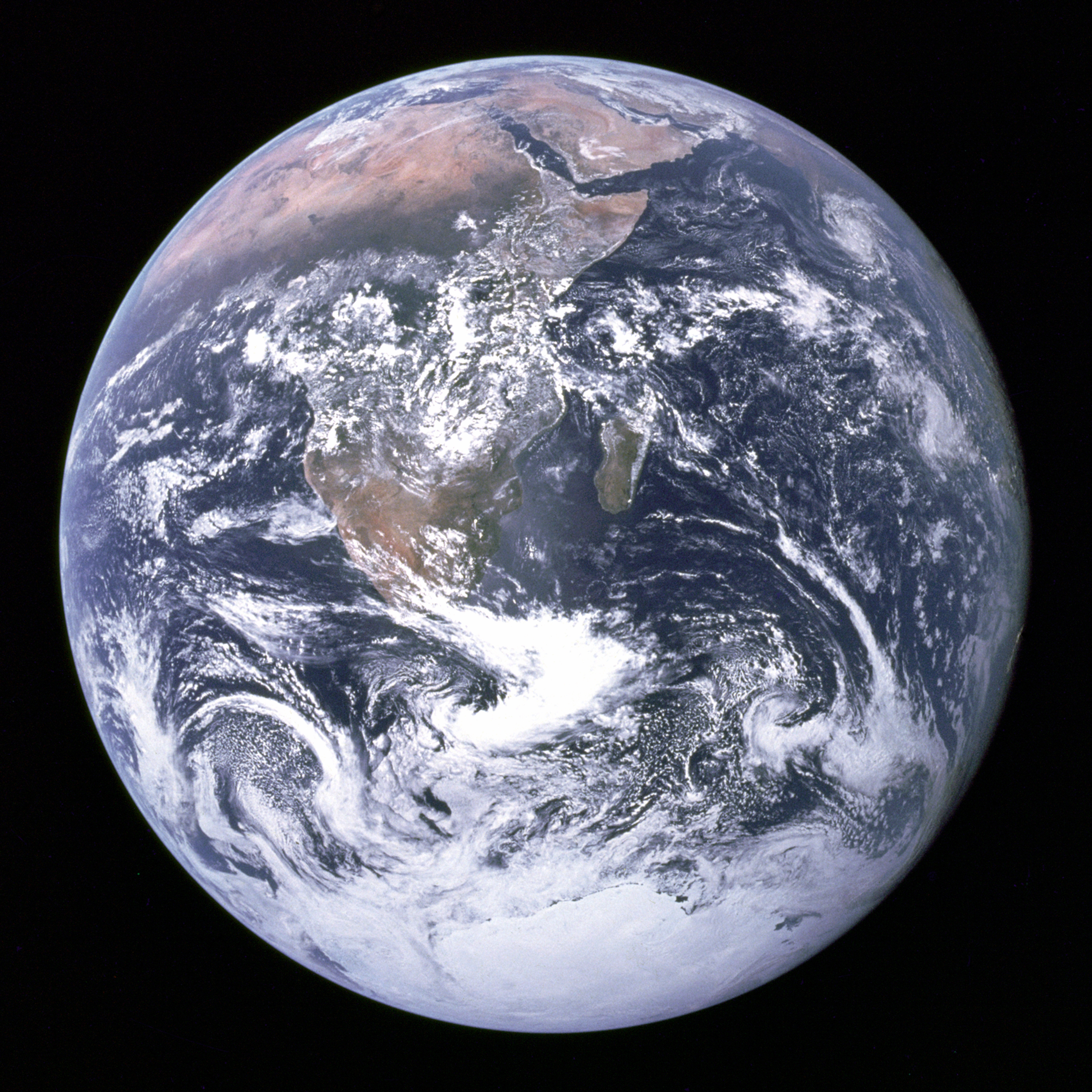
Earth
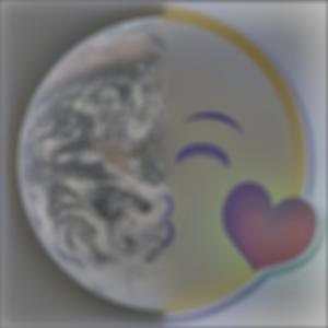
Emoji x Earth
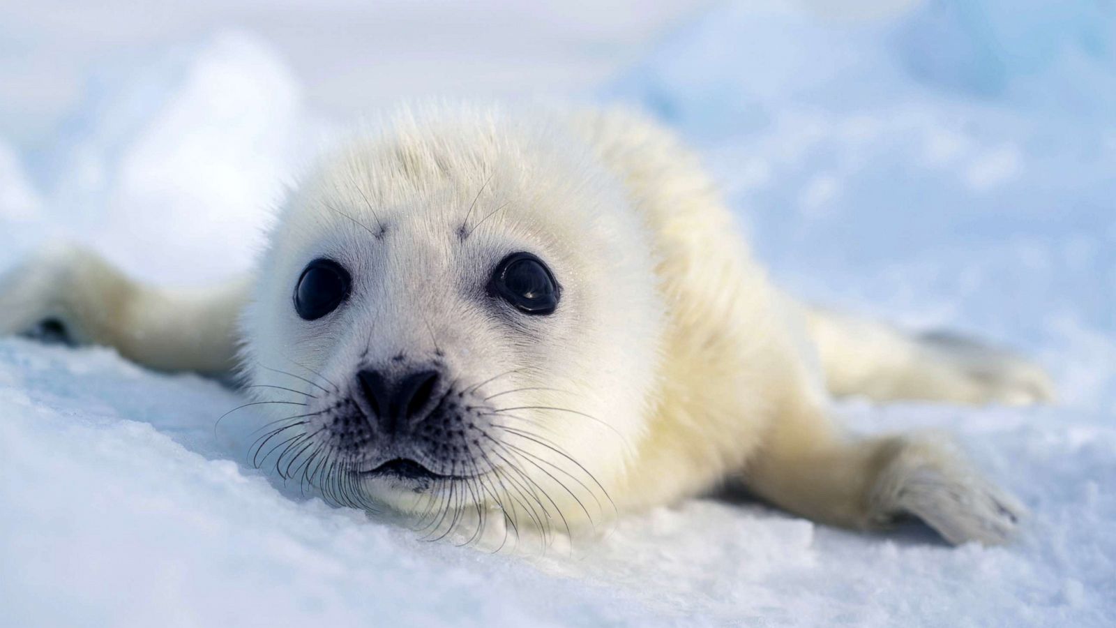
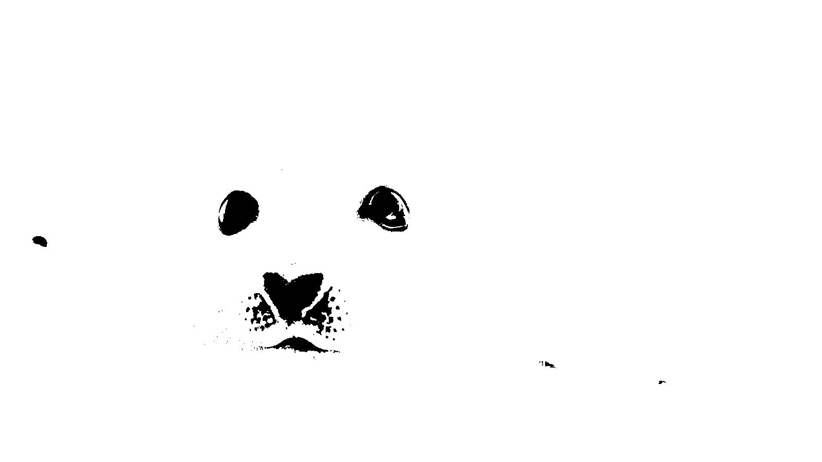
Seal
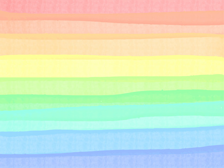
Color
Seal x Color (See the EYES & NOSE!)
Conclusion
In this project, the most important learning for me is to process a picture with different elements in a picture. I was so surprised by the theory behind 2.1, which is sharpening a image without anything more than itself. Also, the power of Gaussian filter can help us do a lot of things, and the math behind it is facinating. Also, one improvement I thought for part 2.4 is a function to resize the images automatically so that two image can blend with each other with less effort.
Bells & Whistles
I implemented 2.4 Multiresolution Blending in color.