CS 194-26
By Won Ryu
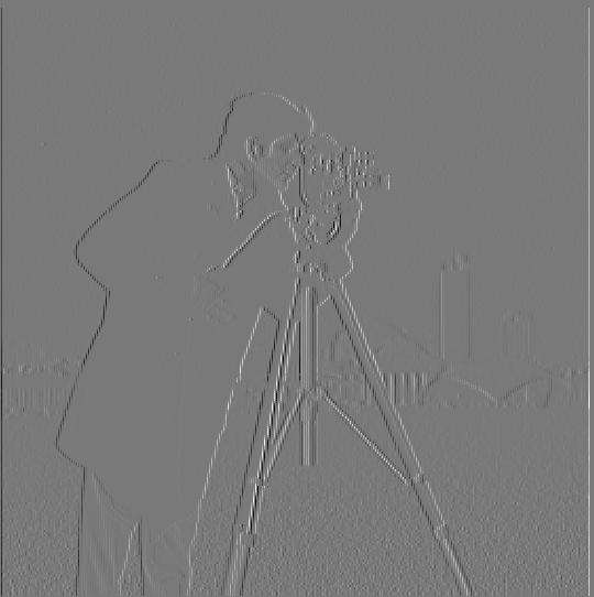
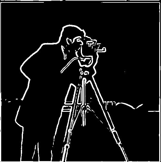
Through convolutions we are able to obtain a gradient magnitude computation. We first obtain the gradient by obtaining the partial derivative with respect to x and partial derivative with respect to y which are the two components of the gradient in the 2d image. The partial derivative with respect to x is obtained by convolving the image with filter [[1, -1]] as the partial derivative with respect to x can be approximated by image(x+1, y) - image(x, y). Similarly, the partial derivative with respect to y is obtained by convolving the image with filter [[1], [-1]] as the partial derivative with respect to y can be approximated by image(x, y+1) - image(x, y). With the partial derivatives computed, we have the gradient of the image which is a 2 dimensional vector. The gradient magnitude can now be computed as it is the magnitude of a 2 dimensional vector which is sqrt(partial_wrt_x^2 + partial_wrt_y^2). With the gradient magnitudes computed, we can also use a threshold and binarize all coordinated with gradient magnitudes that are above or equal to the threshold as 1 and those that aren’t as 0.
partial derivatives with respect to x
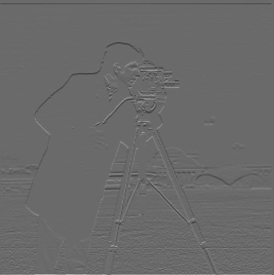
partial derivatives with respect to y
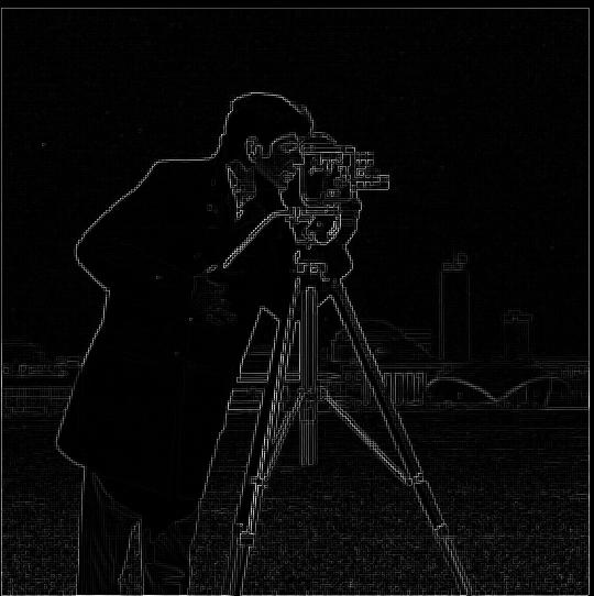
gradient magnitude of image
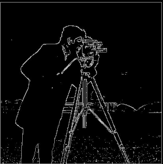
binarized edges where if the magnitude was 0.185 or greater, it was binarized as edge
To reduce noise, we’ll first smoothen the picture by convolving the original image with gaussian and then following the procedure in part 1.1.
Now, we see differences of noise being significantly reduced as we no longer see the grainy grass that was causing salt and pepper noise and also the edges of the human and the camera is a lot more continuous and smoother. Another difference was that now the threshold in which we would classify as an edge needed to be lowered to classify edges.
For efficiency, we’ll take advantage of the associative property of convolutions and create partial derivative of gaussian with respect to x and y that we can use as filters. In this way, we have one filter instead of two.


The edge image ends up becoming the same results as before as it follows the mathematical associativity property.
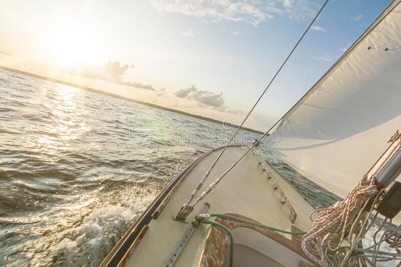
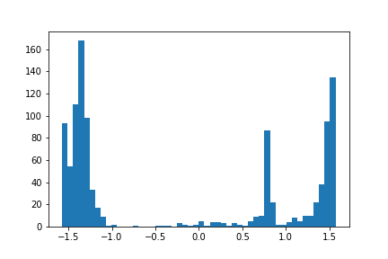
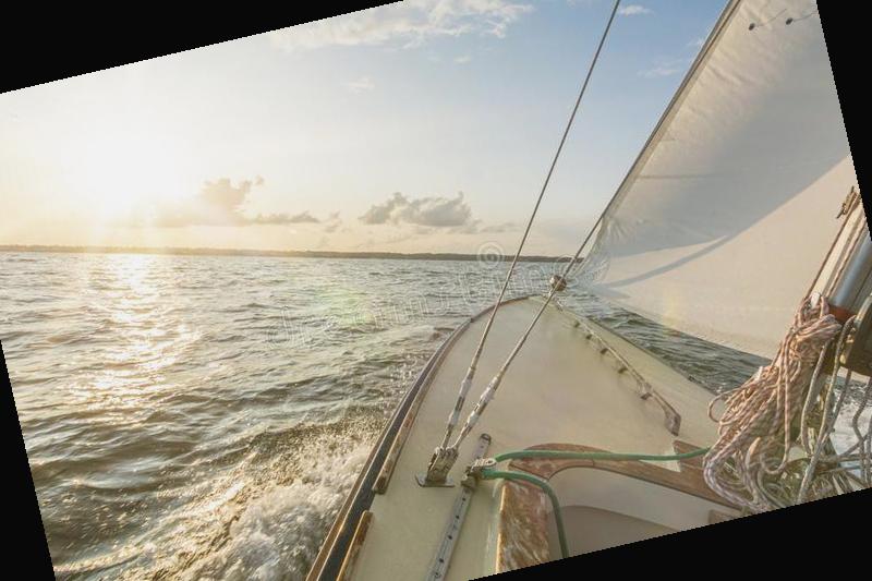
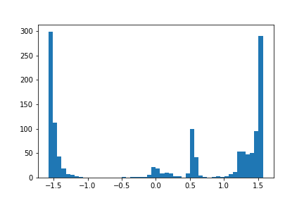
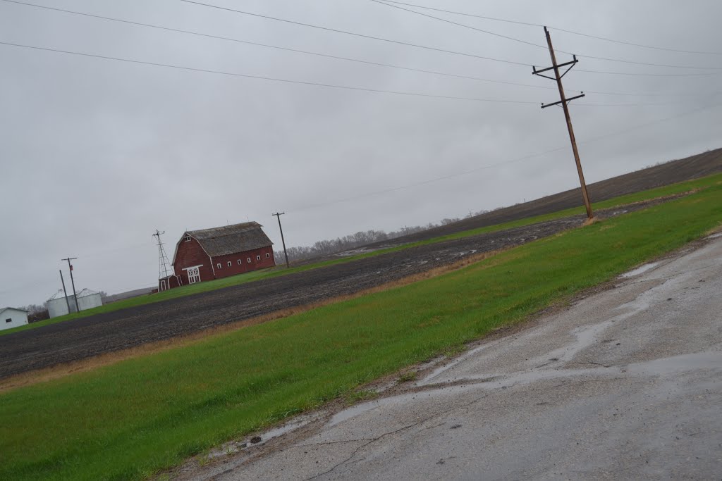
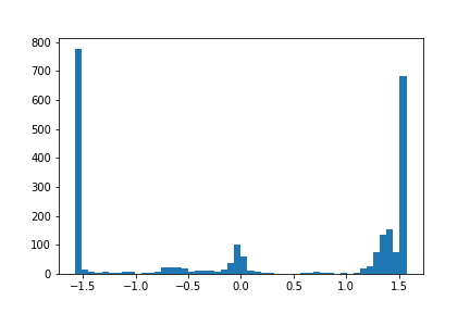
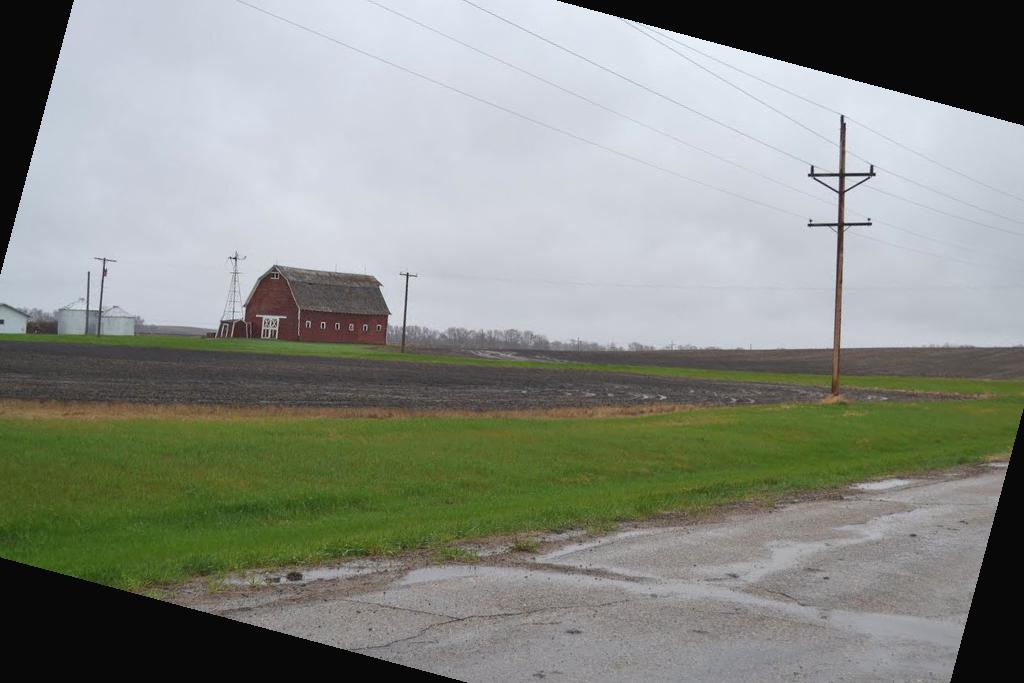
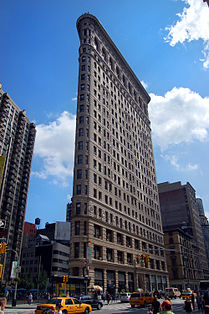
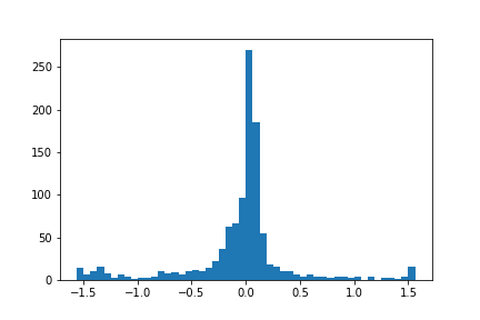
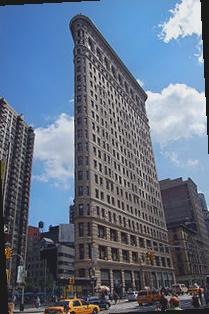
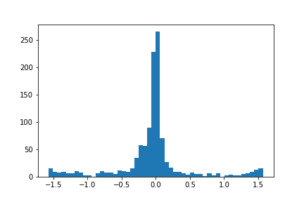
Now we will do image straightening by maximizing the number of horizontal and vertical edges. We’ll rotate the image in a range of angles and keep the angle that maximizes the number of edges that are either horizontal or vertical.
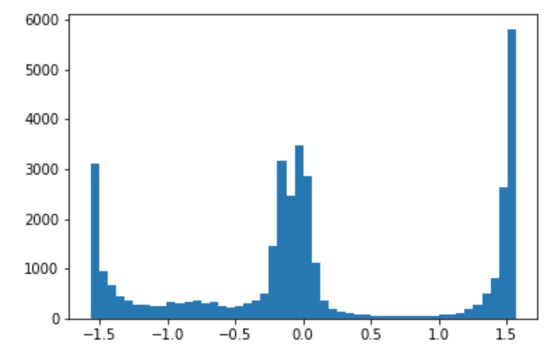
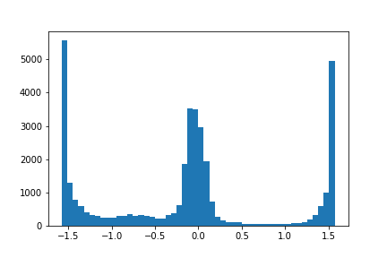
Optimal degree rotation: -3
Optimal degree rotation: 13
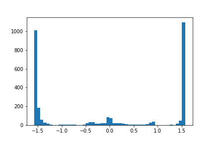
Optimal degree rotation: -15
As seen in the straightened image, cars are driving at an angle in New York City which is a flat city which implies the straightening failed as the algorithm tried to align the building as vertical as possible as those had the most edges.
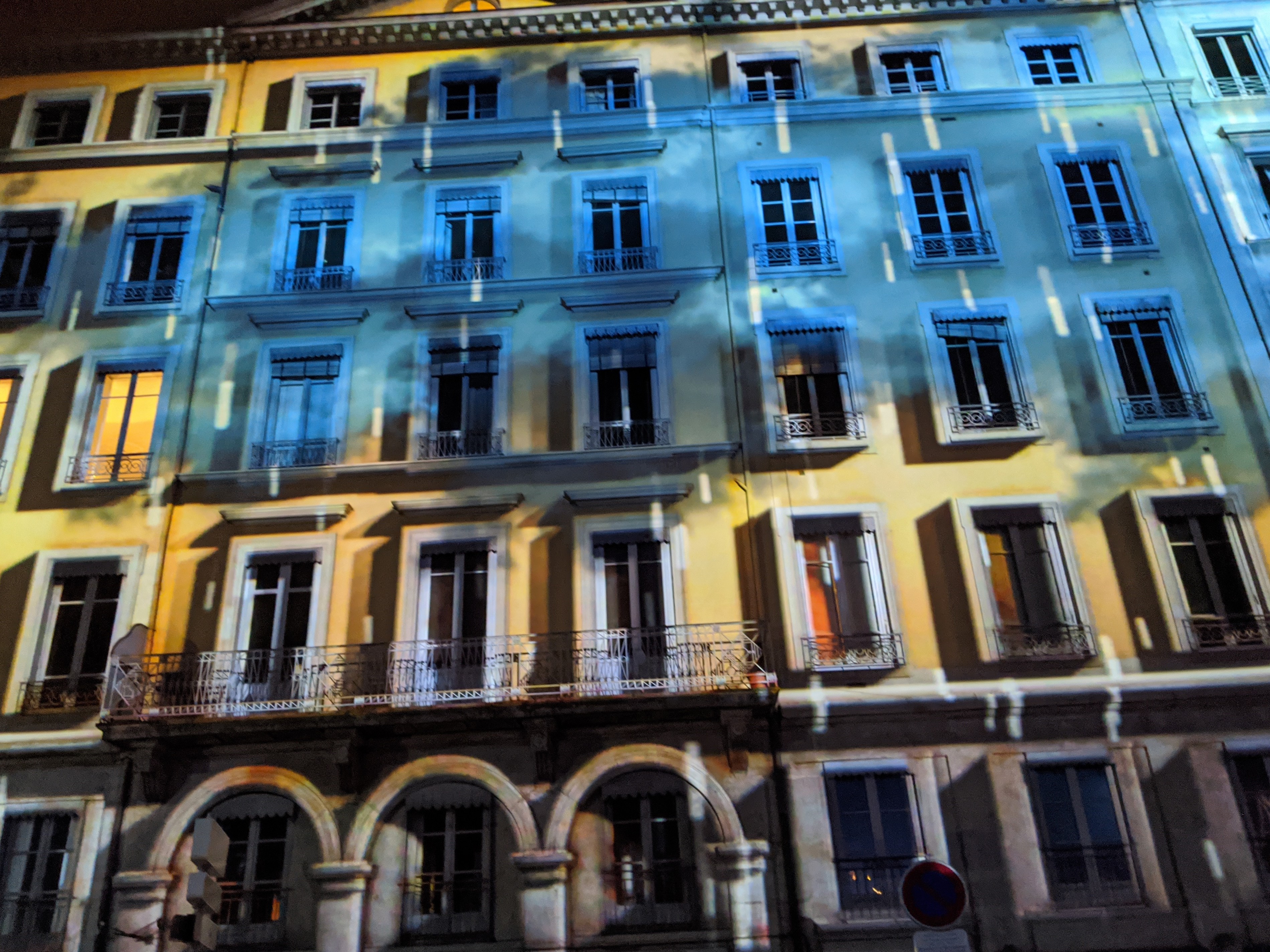
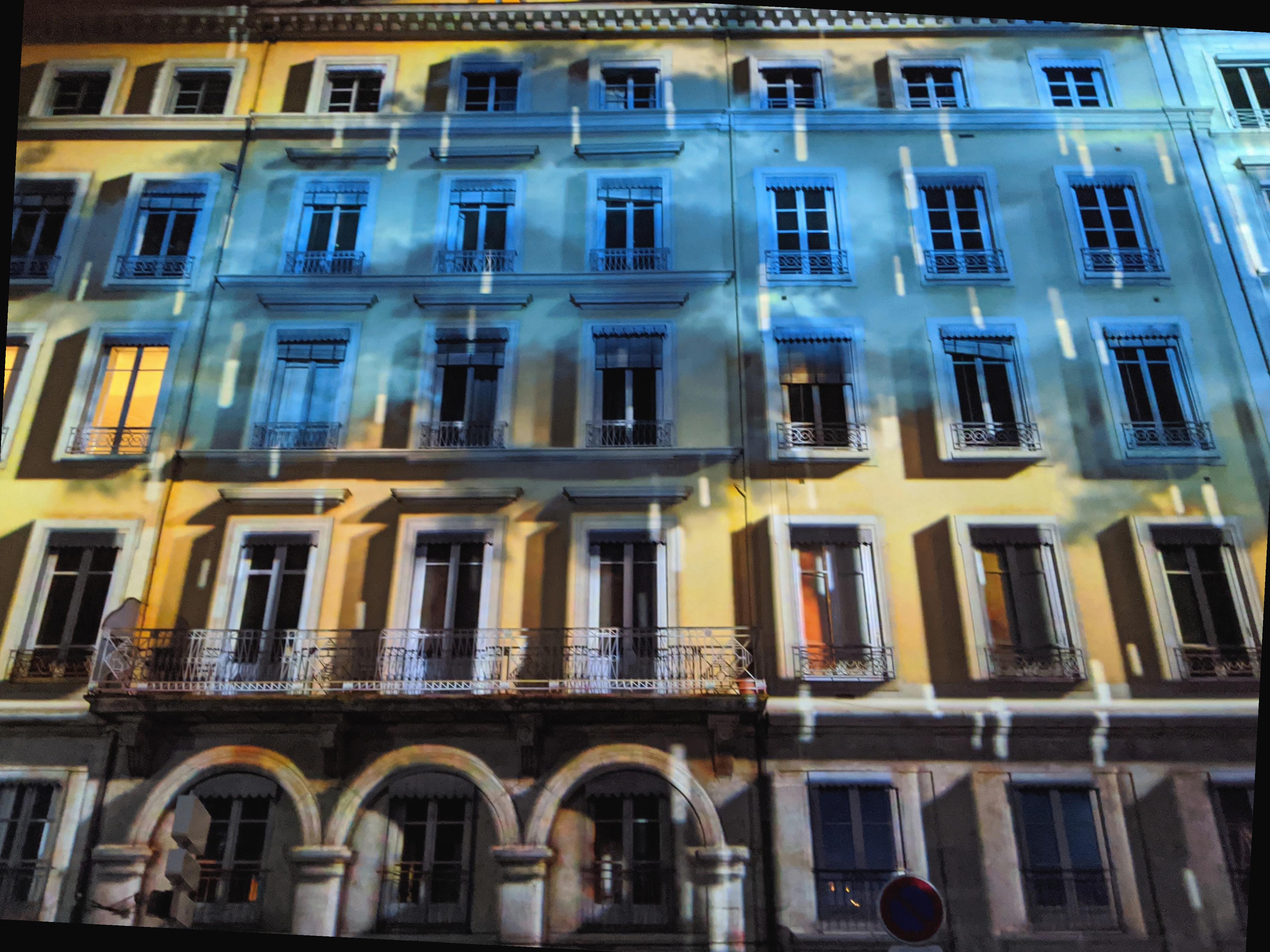
These images were sharpened by having their high frequencies added more proportional by an alpha value. The high frequencies of the images were found by taking the original image and subtracting the low frequencies of the image.
Alpha: 0.5
unsharpened:
sharpened:
unsharpened:
sharpened:
For evaluation of this sharpening method, we blurred an image and then resharpened it using this method. As visible, this sharpening method merely makes the image appear sharper but doesn’t add the high frequencies we lost when blurring and therefore can not be as sharp as the original image.
Original image:
Blurred out:
Resharpened:
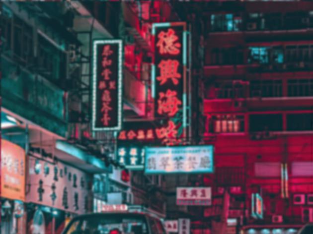
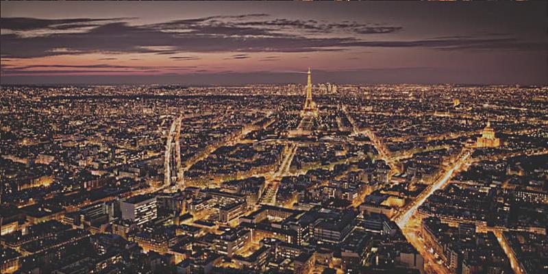
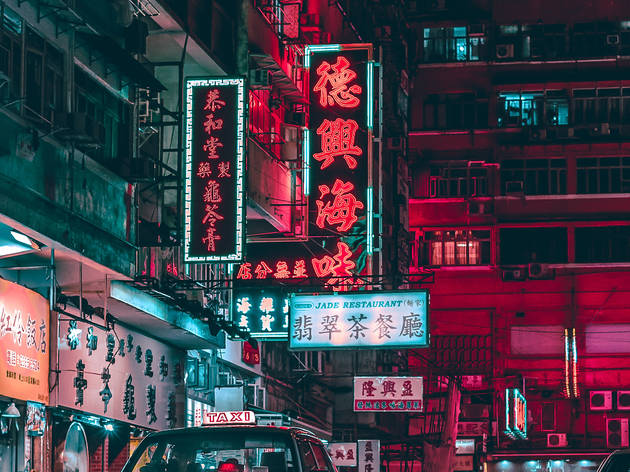
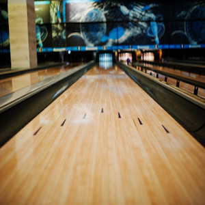
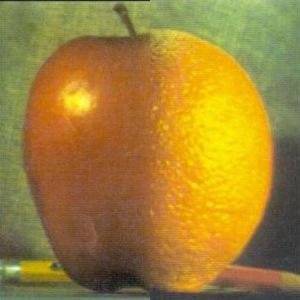
We can also create hybrid images by aligning two images, getting the high frequencies of one image, the low frequencies of the other, then adding those two images together. Then from a far we see the image with the low frequency and up close we see the image with the high frequency.
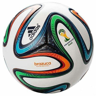
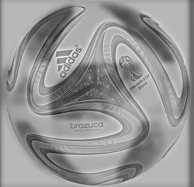
Image for low frequency:
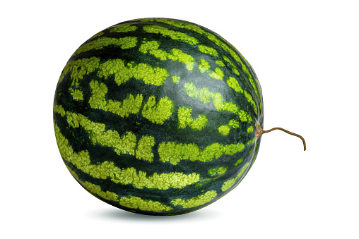
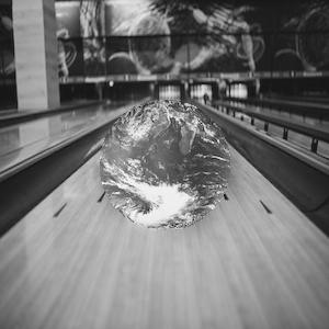
Image for high frequency:
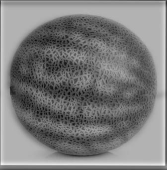
Hybrid:
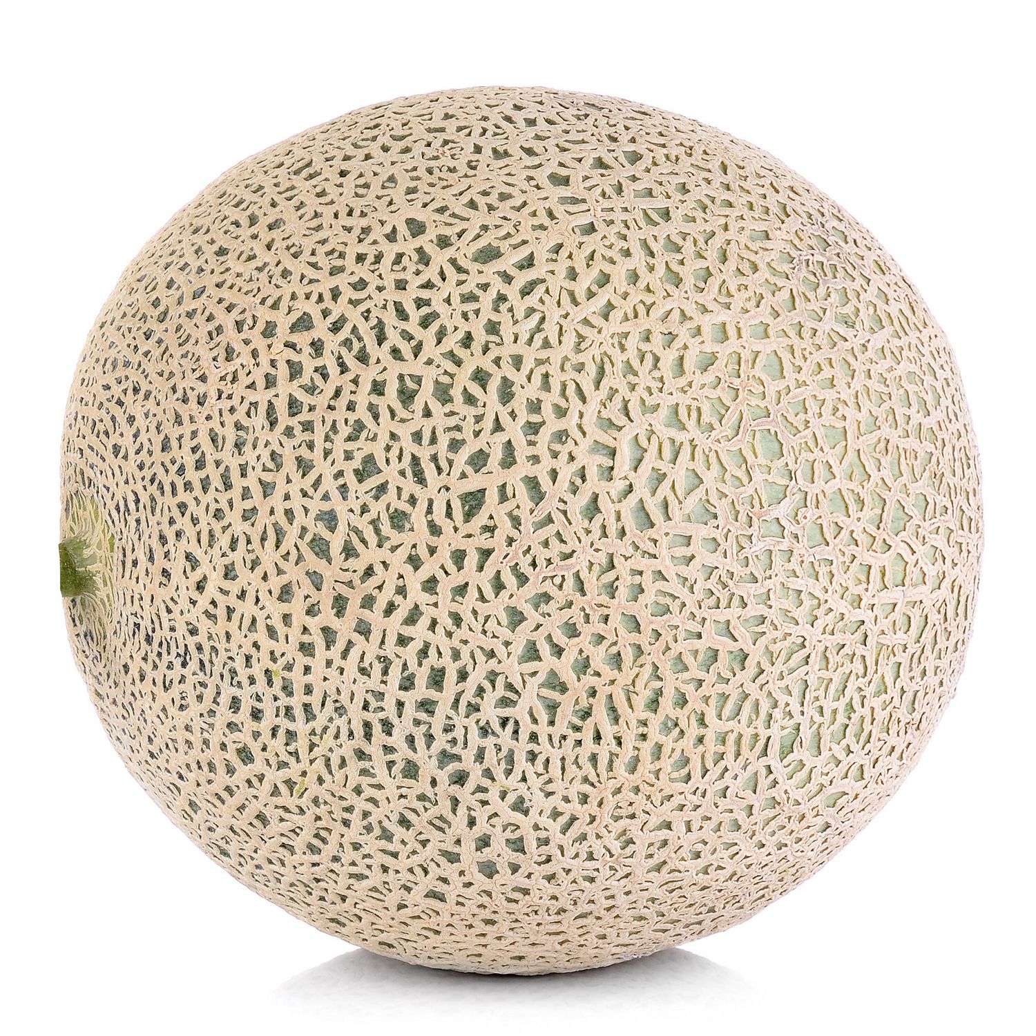
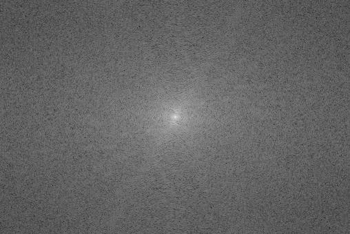
Log magnitude of the Fourier transformation of original cantaloupe
Log magnitude of the Fourier transformation of original watermelon
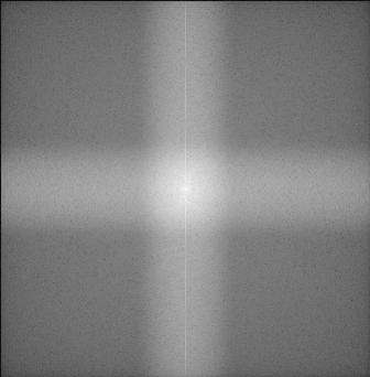
Log magnitude of the Fourier transformation of high frequency of cantaloupe
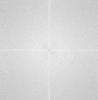
Log magnitude of the Fourier transformation of low frequency of watermelon
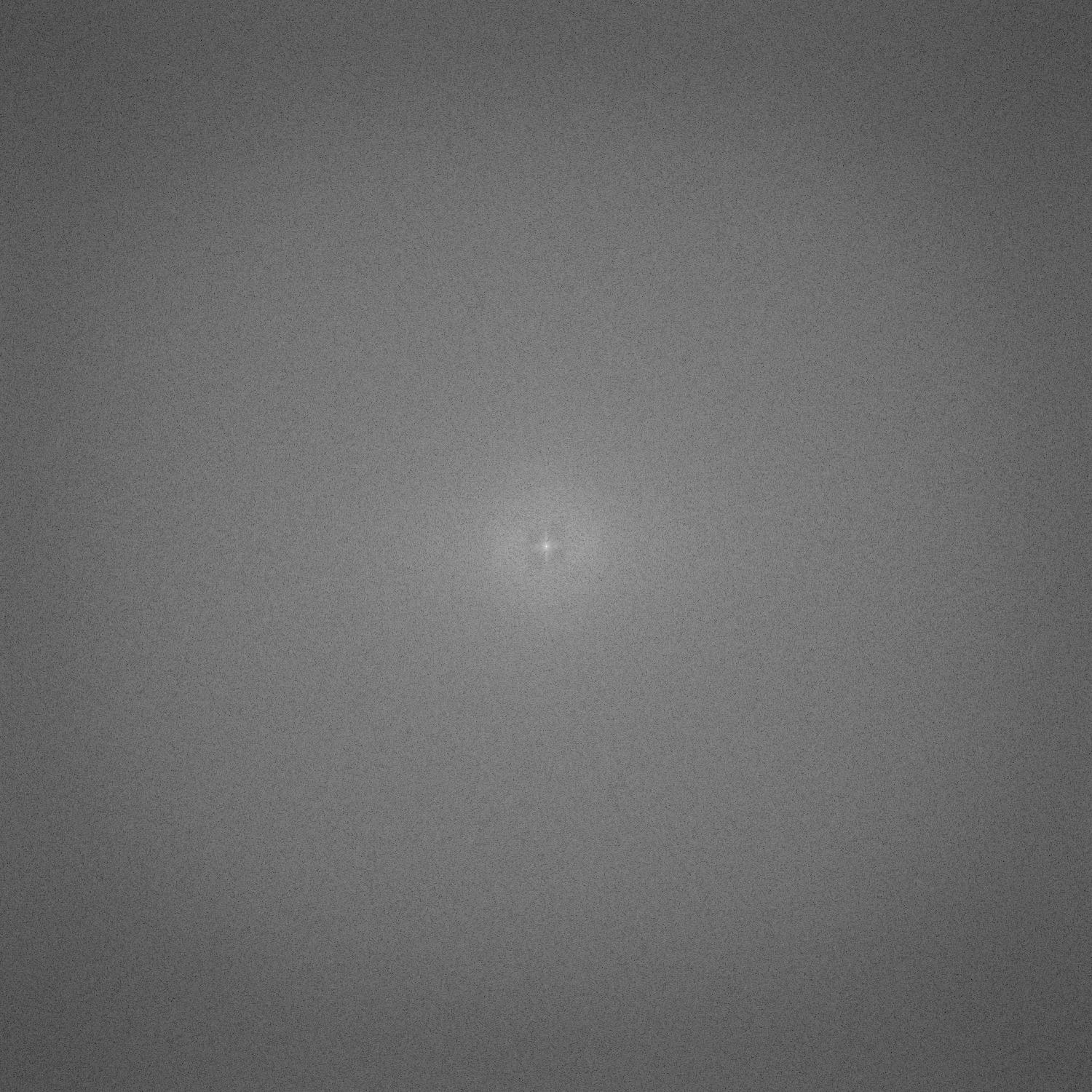
Log magnitude of the Fourier transformation of hybrid image
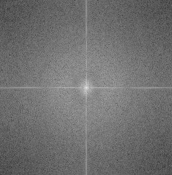
Image for low frequency:
Image for high frequency:
Hybrid:
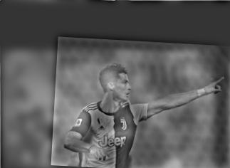
As seen in this failure case, the hybrid images only work when the images are able to be well aligned. In these two separate images, Messi and Ronaldo are in different poses which makes hybrid images with pictures not as effective.
Image for low frequency:
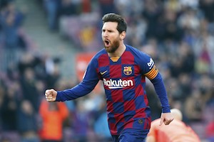
Image for high frequency:

Hybrid:
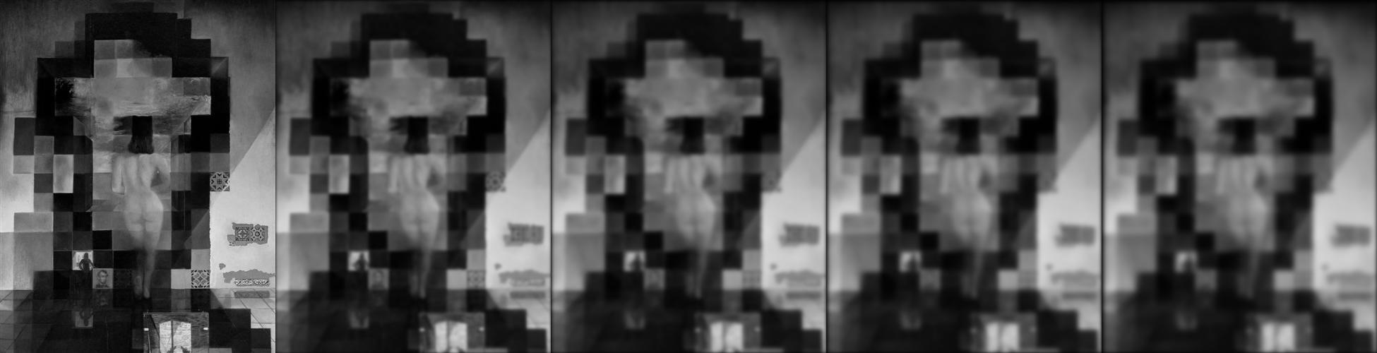
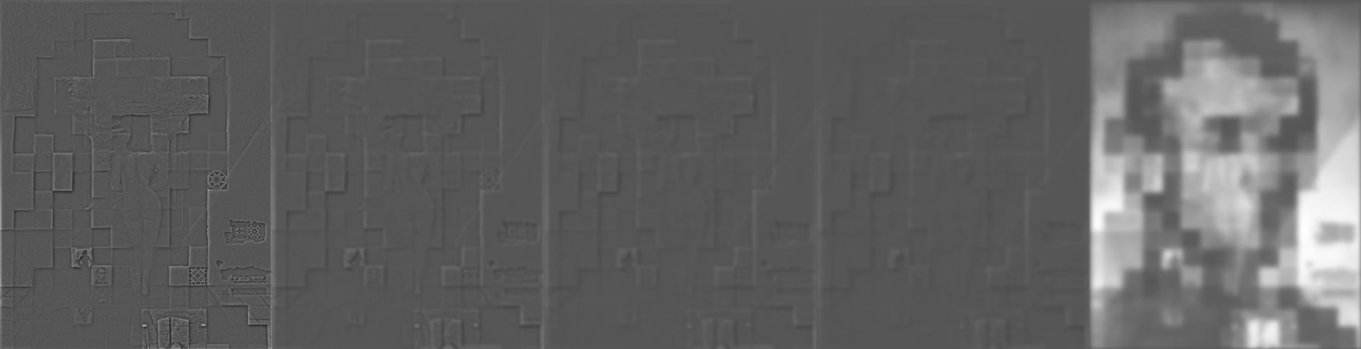
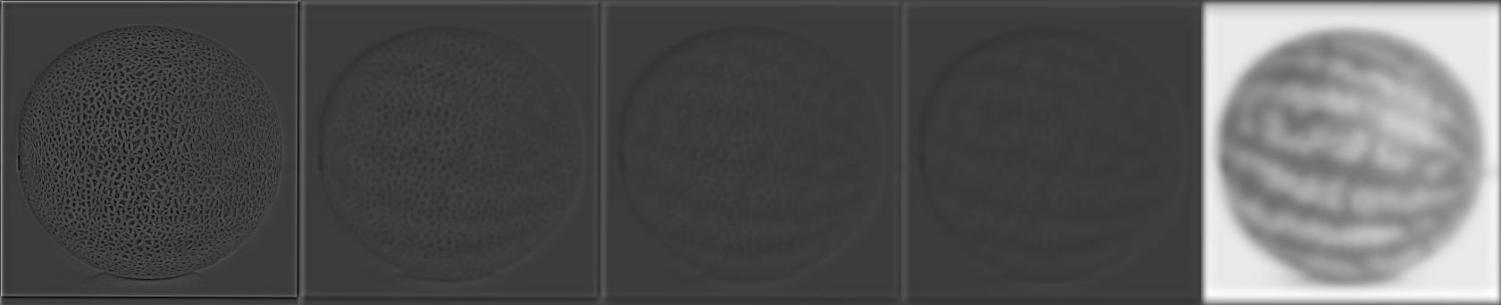
In this part, a Gaussian and Laplacian stack was implemented. The gaussian stack was implemented by starting with the original image as the first layer, each layer was found by convolving the previous layer with a gaussian. The laplacian stack was implemented where each layer of the laplacian stack was the difference between the same layer at the gaussian and the layer after that. The last layer of the laplacian was just the last layer of the gaussian.
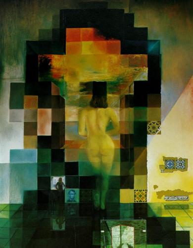
Gaussian stack:
Laplacian stack:
Gaussian stack:

Laplacian stack:
Multiresolution Blending
Two images were blended seamlessly using multiresolution blending. The images were blended similarly to Burt and Adelson’s approach in 1983.
Image 1:

Image 2:
Mask:

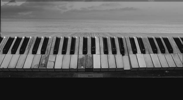
Blended:
Laplacian stack of sea:

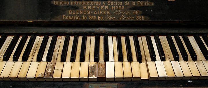
Laplacian stack of piano:

Gaussian Stack of mask:

Masked laplacian of sea:

Masked laplacian of piano:

Merged:

Image 1:

Image 2:

Mask:

Blended:

Image 1:
Image 2:
Mask:

Blended:
I also implemented the multiresolution blending on color by performing the algorithm explained in 2.4 on the 3 color channels separately and storing them separately. Then the result of the blendings on the 3 colors were stacked on top of each other in RGB order.
I learned about the capabilities of filters and convolutions where they can perform everything from calculus, edge detection, smoothening, sharpening, and with those images we can create exciting hybrid images and blended images.