In this project, I learned information behind pictures. The filters and frequencies helps us improve picture quality and make amazing affect on such a picture. It brings us a exciting vision world to explore.

Part 1: Fun with Filters

Part 1.1: Finite Difference Operator

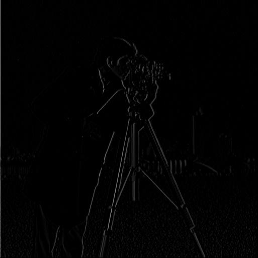
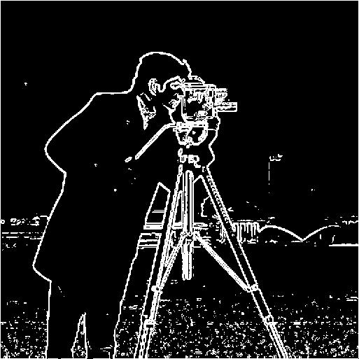
I tried to get an edge image of cameraman. I got partial derivative of cameraman first. As I learned, I calculated convolution grad_x with D_x [[1 ,-1], [0, 0]] to get partial derivative in x I do so for grad_y with D_y [[1, 0] , [-1, 0]].

Next step was getting gradient magnitude image. It is simple: gradient magnitude image equals to sqrt(grad_x^2 + grad_y^2) However there are quite noise (white dots) here. I took a few tries to find good threshold for cameraman:20 But it still looks not prefect.

convolution *grad_y* with D_y [[1, 0] , [-1, 0]]

gradient magnitude image then binarized *grad_binarized*

Part 1.2: Derivative of Gaussian (DoG) Filter

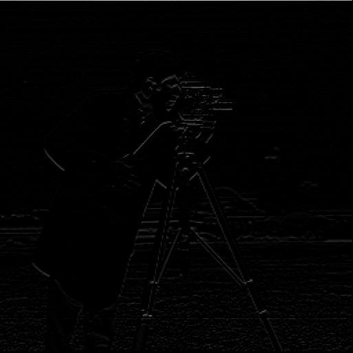
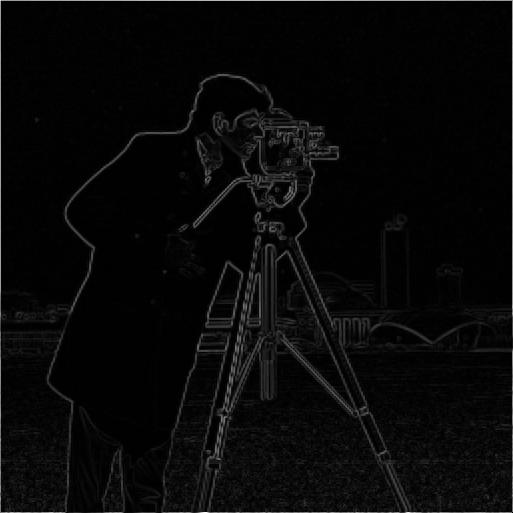
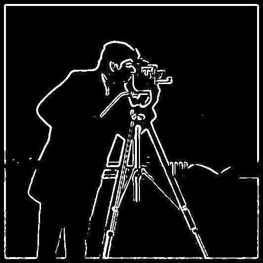
I took sometimes to find the right parameter for GaussianKernel: size = 20 and sigma=1.5. Then I did 2D convolution with Gaussian filter as previous part to get grad_G_binarized. The noise on the bottom almost gone! The entire image looks very clean and tidy. It looks better than grad_binarized, but I couldn't get rid of all white dots: if I did so, the cameraman would lose his arm! Therefore, I tried to get an balance between keeping edges and getting rid of noise.

Also I did signle convolution for 2D Gaussian filter to get its partial derivative in x and y which resulted in derivative filters g_filter_2D_x and g_filter_2D_y then I used them to do convolution with cameraman picture and get grad_DoG_x and grad_DoG_y. Then use gradient magnitude formula and threshold get grad_DoG_binarized. grad_DoG_binarized and grad_G_binarized looks exactly the same one. It showed the derivative of convolution: do derivative then do convolution or do convolution then do derivative got the same result.

gradient magnitude image with a 2D gaussian filter then binarized *out_cameraman_grad_G_binarized*

gradient magnitude image with two derivative of gaussian filter then binarized *out_cameraman_grad_DoG_binarized*

Part 1.3:Image Straightening

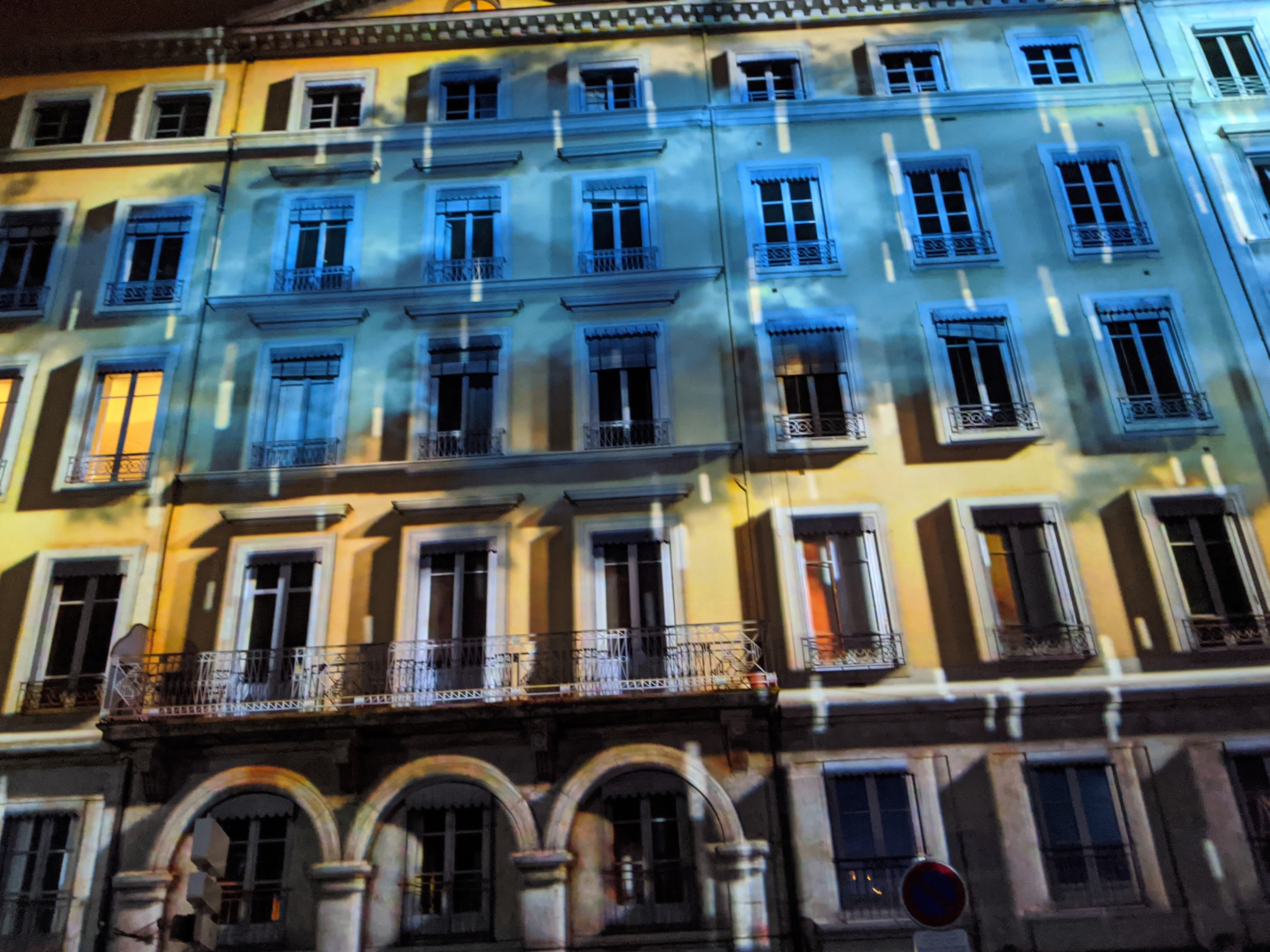
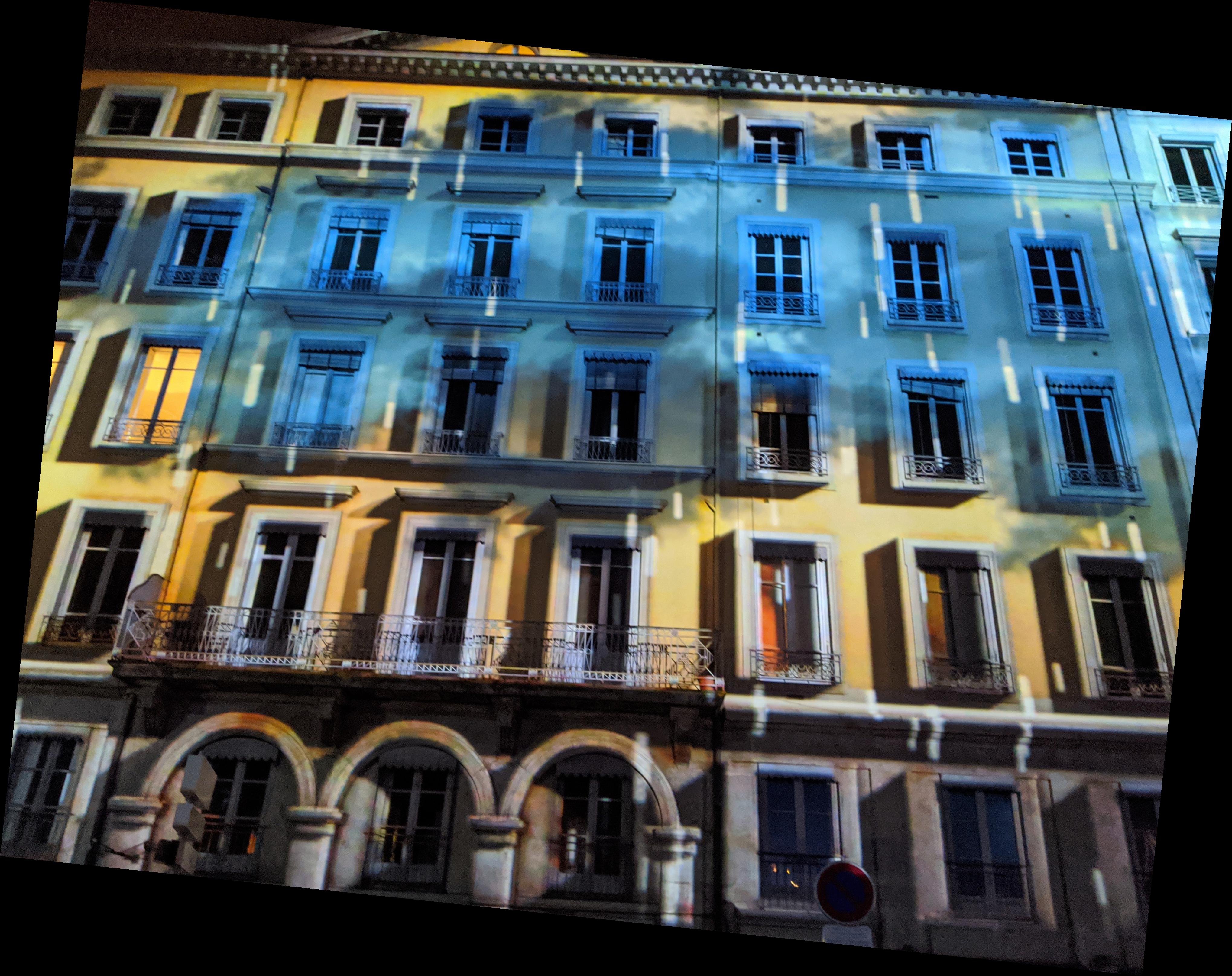
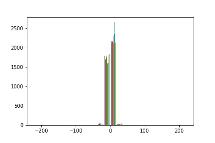
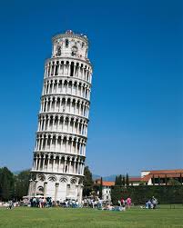
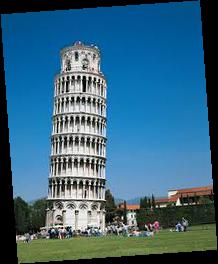
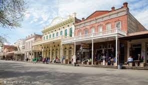
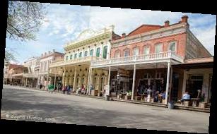
To straighten a image, I can use the partial derivative in x and y of the image to get the angle of any pixel in the image by doing arctan(dy, dx). However, it is important to find whether these pixels are on the edges or not, otherwise the rotation would be wrong. My solution is check gradient magnitude to make sure these pixels' gradient magnitude over my threshold. Also, border need to cropped, which would be counted as fake edge in my algorithm.

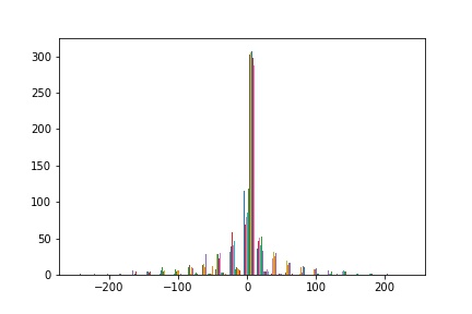
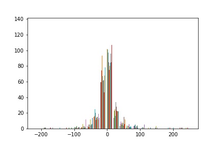
From histogram, it is easy to that if the image is straightened, the peaks on left and right of the histogram should almost be balanced. If the image is not straightened such as Scramento, it has two obvious highest peaks which has different height.

Histogram of angle in straightened facade

Straightened Torre pendente di Pinsa with 4 degree

Histogram of angle in straightened Torre pendente di Pinsa

Histogram of angle in straightened Scramento

Part 2: Fun with Frequencies!

Part 2.1: Image "Sharpening"

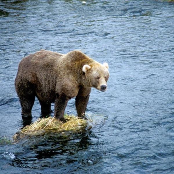
How to sharpen image? For human, we feel "sharp" when image has much high frequencies or less low frequencies. Here is how to do that: create a unit impulse which is a matrix with same shape as Gaussian filter which has all zero except its center is one. Gaussian filter has low frequencies. So I got a laplacian of Gaussian with formula ((alpha + 1) * laplacian - alpha * Gaussian filter) which get more high frequencies and less low frequencies by increasing alpha. After tweak a little bit, I use size=10, sigma = 10 and alpha = 2 as my parameters to do sharpening.

Compare to the original image and the sharpened image, they are quite different. Only if you look them from far away, you will thought they are the same. Because blur can normalize the pixel which means that it lose some low frequencies value. Therefore, the sharpened image looks still blurry. On the other hand, sharpening made edges which were not obvious in original be more obvious since sharpening add duplicate high frequencies.

Part 2.2: Hybrid Images"

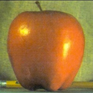
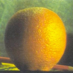
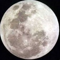
To hybrid images, I aligned two pictures a and b. Then I got high frequencies from picture b by substracting original image b with Gaussian filtered image b. At last, I added the high frequencies from b to Gaussian filtered image a.

This hybrid image has worked not so well. I can see Derek from far away and I can see nutmeg a little bit if I getting closer.

This hybrid image is ok. I can see Justin Bieber from far away and I can see Trump clearly if I getting closer. It is a funny hybrid image by the way.

This hybrid image is failed. I can see lion from far away and I cannot see tiger clearly if I getting closer.

frequency analysis

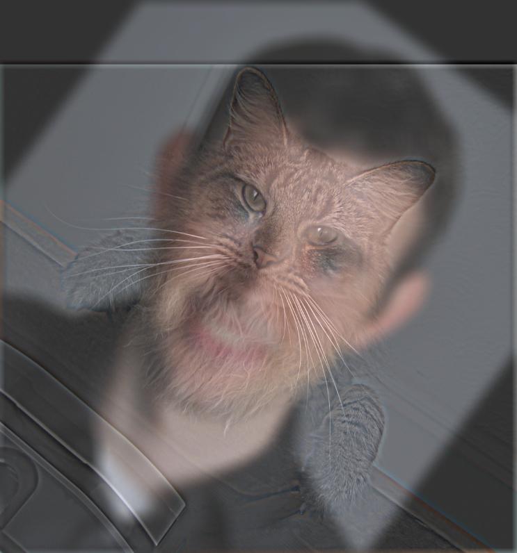
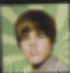
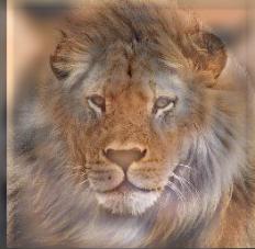
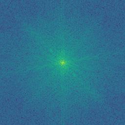
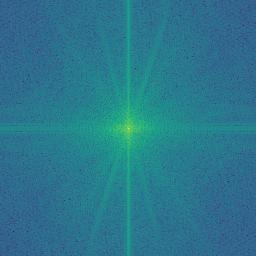
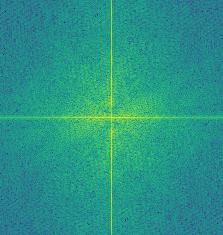
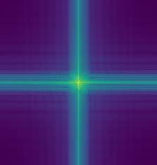
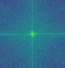
It is clear to see that The FFT of low frequencies from Justin Bieber has purple area because I used high sigma for him so that no much spectrum on four corner of it. It is clear to see that The FFT of high frequencies from Trump has lighter green light because it keeps high frequencies which bring more spectrum to it. At last, it is very clear to see the green cross in the hybrid FFT. Because Justin Bieber's low frequencies and Trump's high frequencies can add each other so it looks no so light like Trump's light or no so purple like Justin Bieber's FFT corner.

The FFT of low frequencies from Justin Bieber.

The FFT of hybrid Justin Bieber and Trump.

Part 2.3: Gaussian and Laplacian Stacks

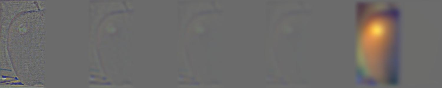
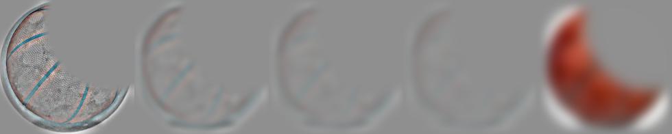
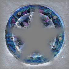
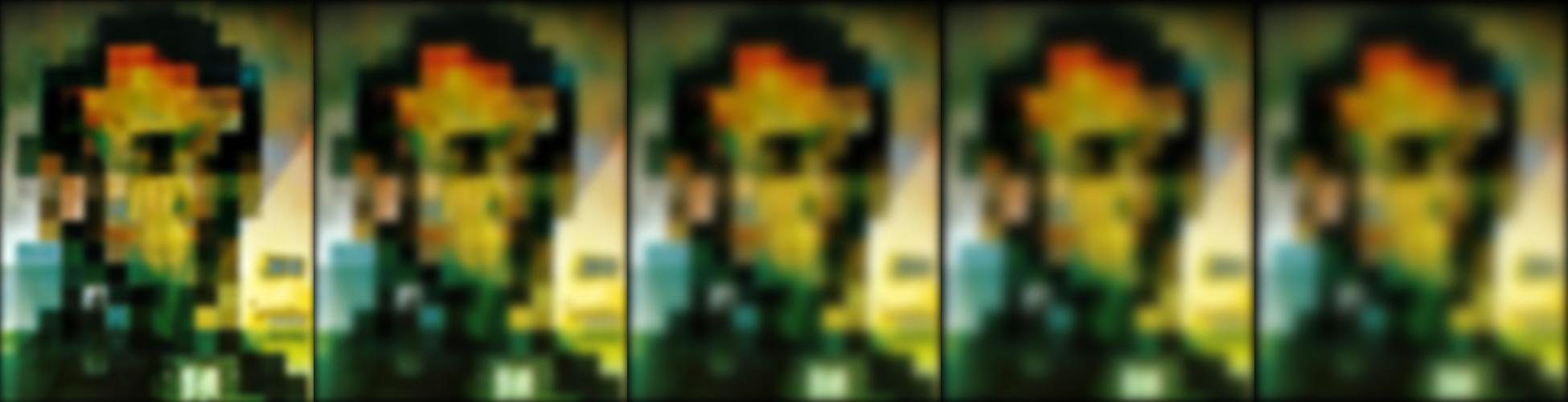
Since I got Gaussian filter in previous part, it is easy to think of do that multiple times like pyramid in project1. However, the size of image would not change in Gaussian and Laplacian Stacks. The first part is Gaussian stack, it filtered image with low frequencies again and again. Then I built Laplacian stack started from the first filtered image by Gaussian filter and went throught it. Laplacian substracted Gaussian filtered image again and again which resulted in high frequencies.

This Gaussian stack clearly shows that Lincoln becomes clear through Gaussian stack. The woman in the image becomes hard to see.

This Laplacian stack clearly shows that the woman in image becomes blurry through Laplacian stack. The woman in the image becomes hard to see. Compare to the woman, Lincoln becomes clear a little bit even the edge got blurry.

This Gaussian stack clearly shows that Trump becomes blurry through Gaussian stack.

This Laplacian stack clearly shows that the Trump in image is very sharp at the beginning. It becomes blurry through Laplacian stack.

Part 2.4: Multiresolution Blending (a.k.a. the oraple!)

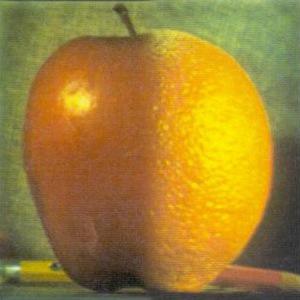
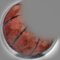
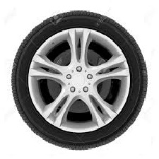
With http://persci.mit.edu/pub_pdfs/spline83.pdf page14, I can use a mask to put one image on another image with very smooth boundary. I made some paint with Windows Paint. It is easy to how image got filter in LS.

Bells & Whistles