1 Overview
In this project, we are going to explore edge detector, image sharpening, hybrid images and image blending. All of these functions are achieved by appling filters on images using convolution.
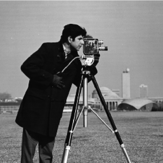
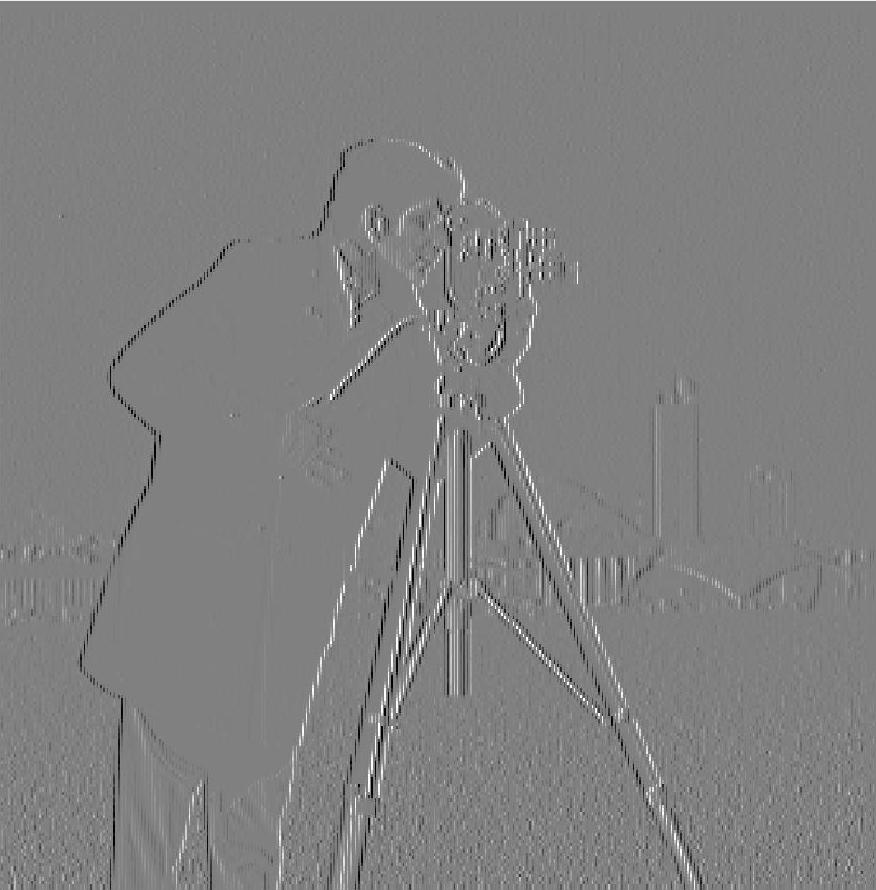
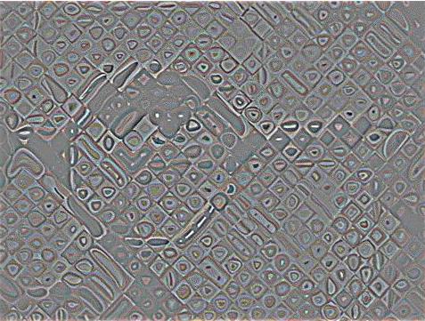
2 Edge Detector (gradient filter)
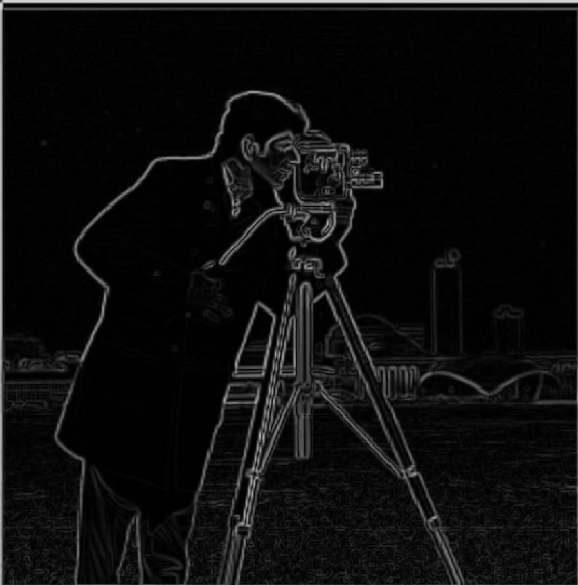
As we know, a clear edge means there's a great difference between adjacent pixels, which also means there's a great gradient. To detect edges, we convolute the image matrix by x_gradient matrix [1 -1] and y_gradient matrix [1; -1], and the result would be the gradient on x direction at all pixels and the gradient on y direction at all pixels (2nd & 3rd image below). To view the overall edge/gradient, we calculate the magnitude of the combined gradient vector, which is (x_gradient^2+y_gradient^2)^0.5.
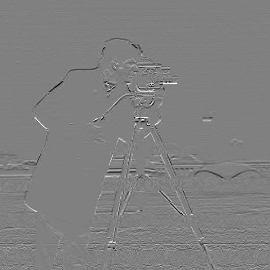
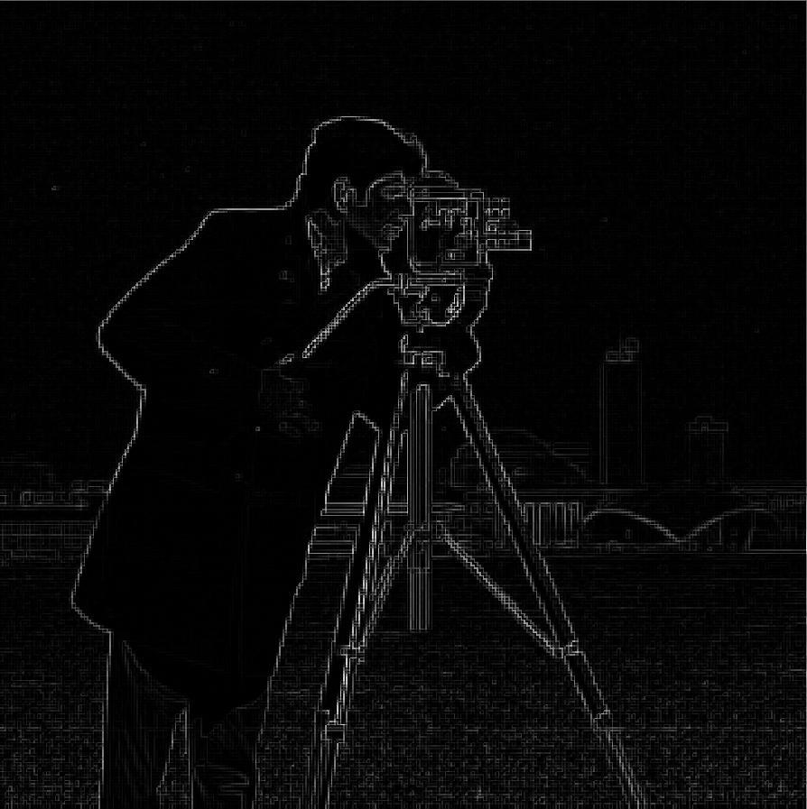
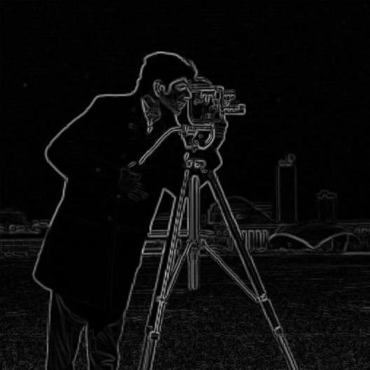
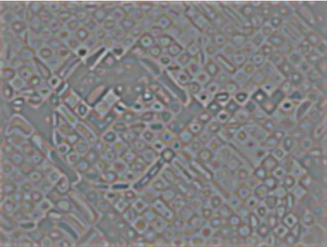
2.1 Improvement: Use Gaussian Filter (low frequency filter) first to reduce noise
We notice that in the result of last part, the edges are not smooth. To reduce the noise, we can convolute the image with Gaussian filter first, then convolute the result with the gradient filters. From the images below, we can see Gaussian filter did reduce the noise and make edges smoother. Another way to do this is by applying the gradient filter on Gaussian filter, then apply the combined filter onto the image. The two methods produce the same result because of the property of convolution.
.
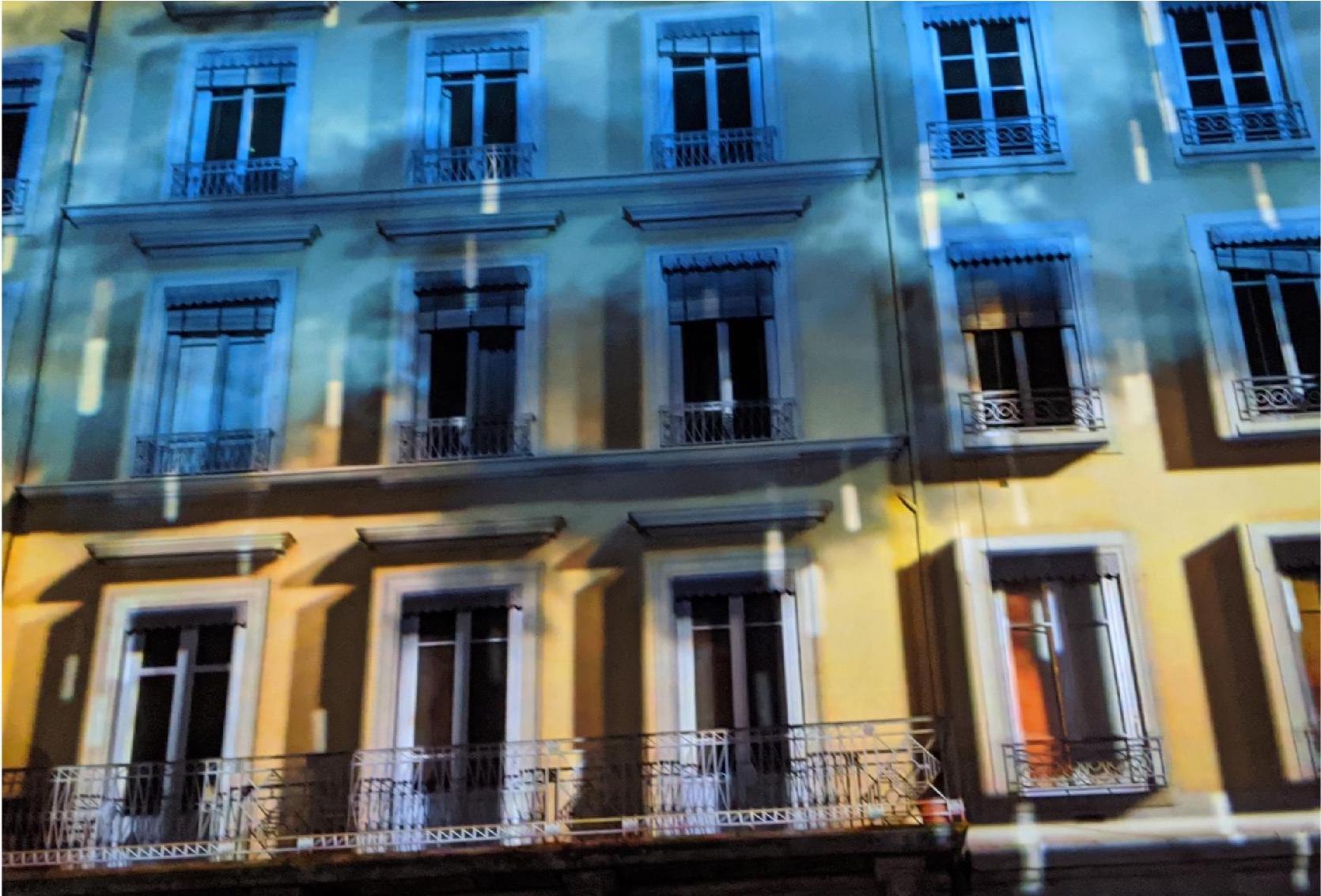
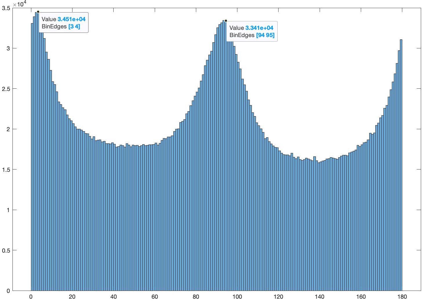
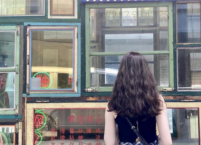
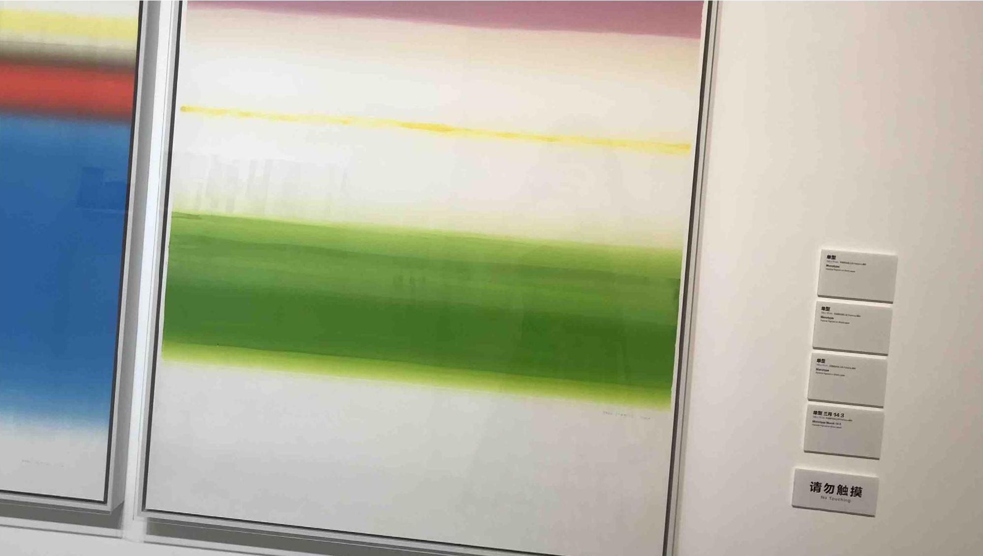
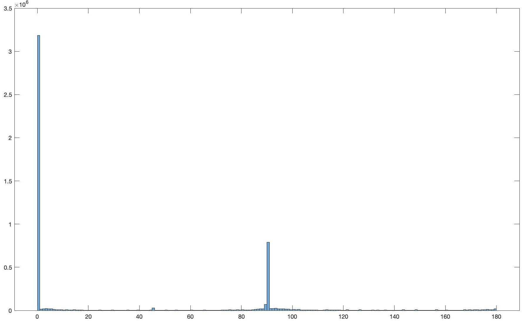
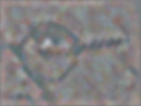
2.2 Application: Image Straightening
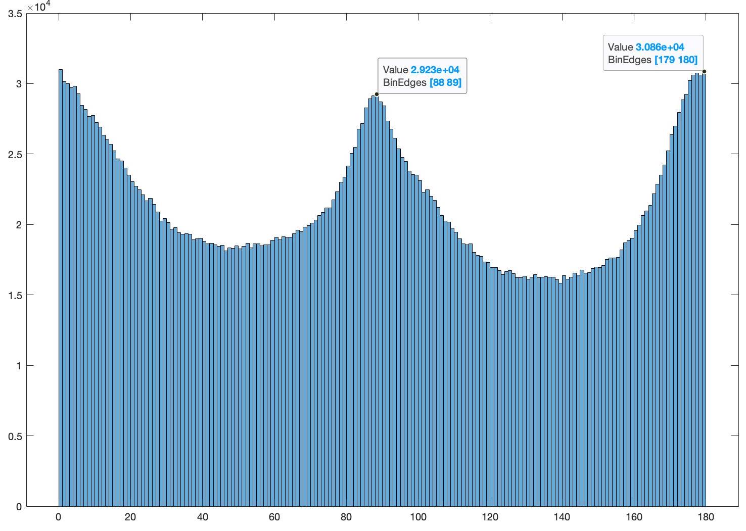
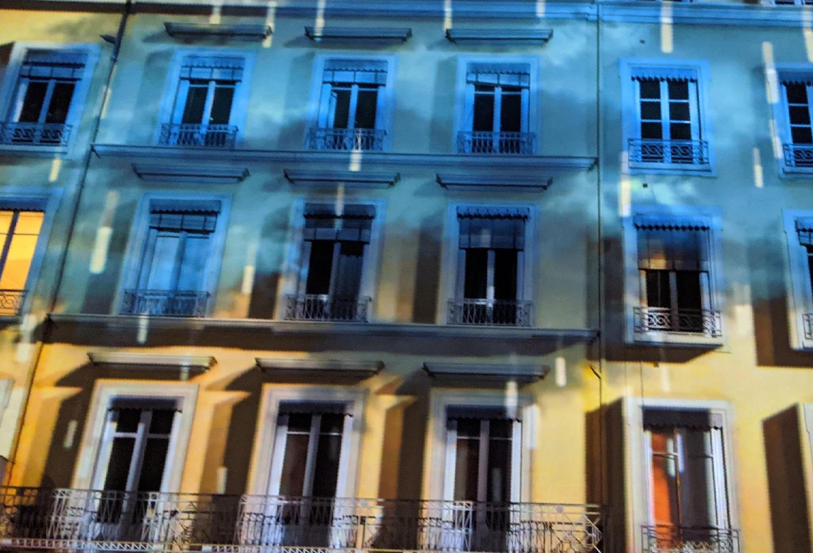
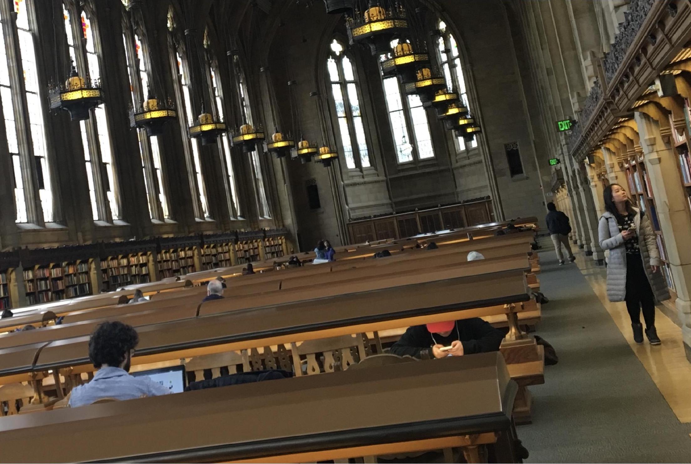
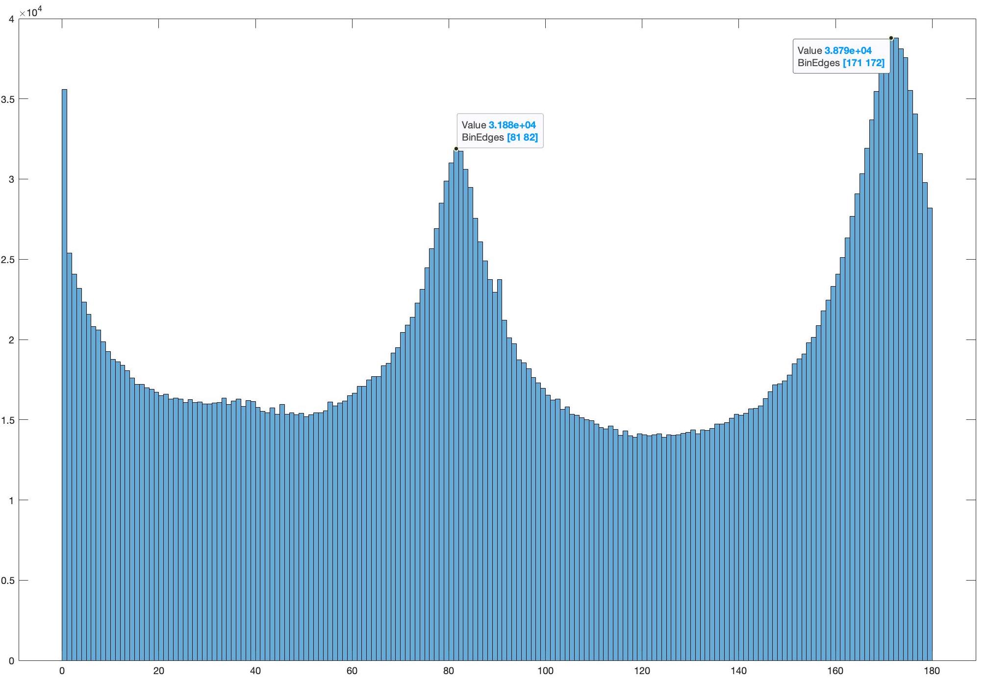
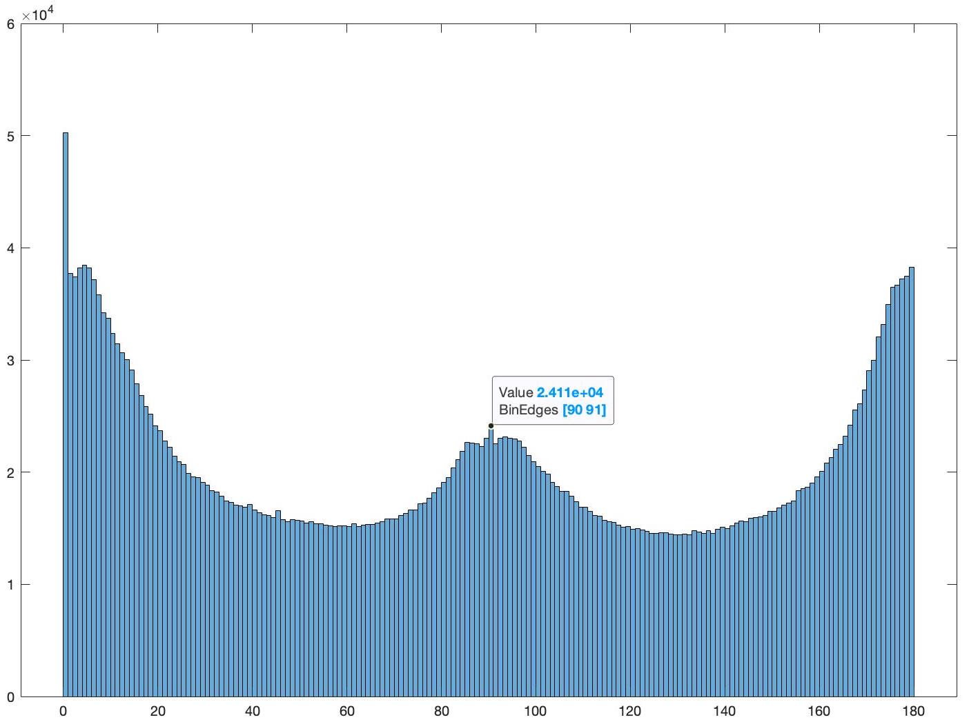
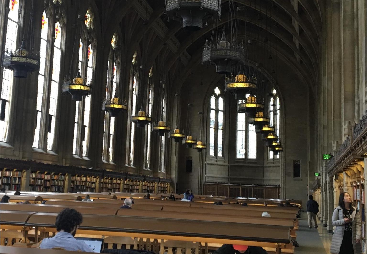
One application to utilize edges is straightening an image. By maximizing the number of vertical and horizontal edges, we can rotate the image to be straight. Below are some examples with original image, its orientation histogram, straightening image and its orientation image. To reduce the effects caused by black edges produced during the rotation process, we crop the result image and only consider the center part. During the practice, however, the number of 0 angles is not accurate, because for a large area with an identical color, the angles for all pixels would be 0 due to 0 y-direction gradient. Therefore, we want to focus more on number of 90 degree angles. Furthermore, we realized that besides the exact number, the peak is also a good indicator.
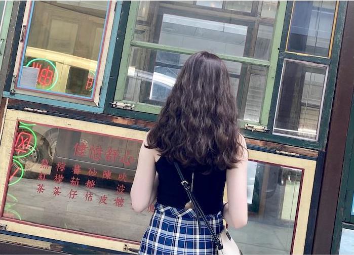

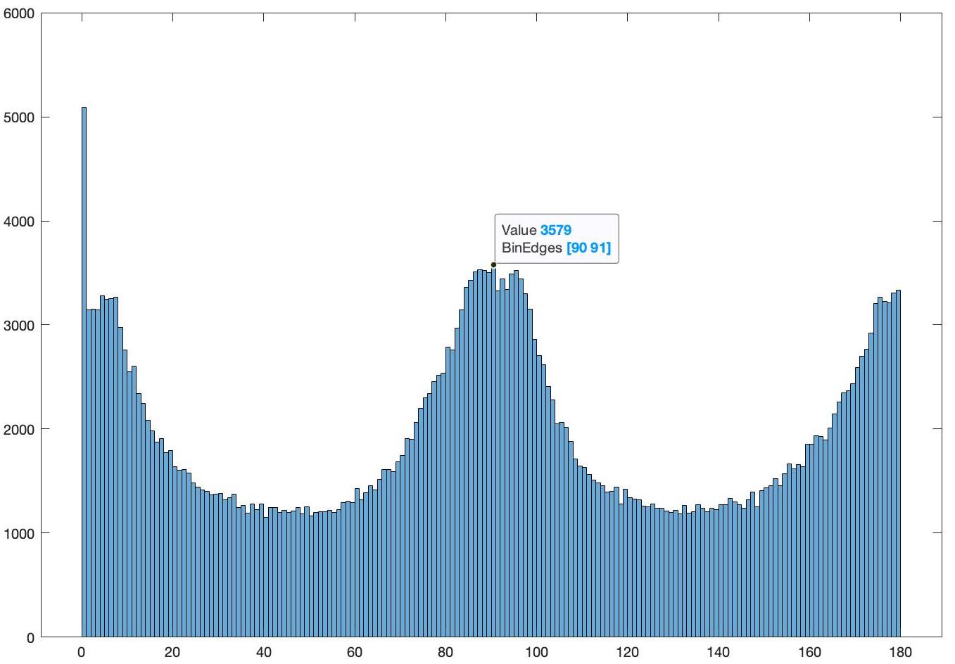
Failure Case:
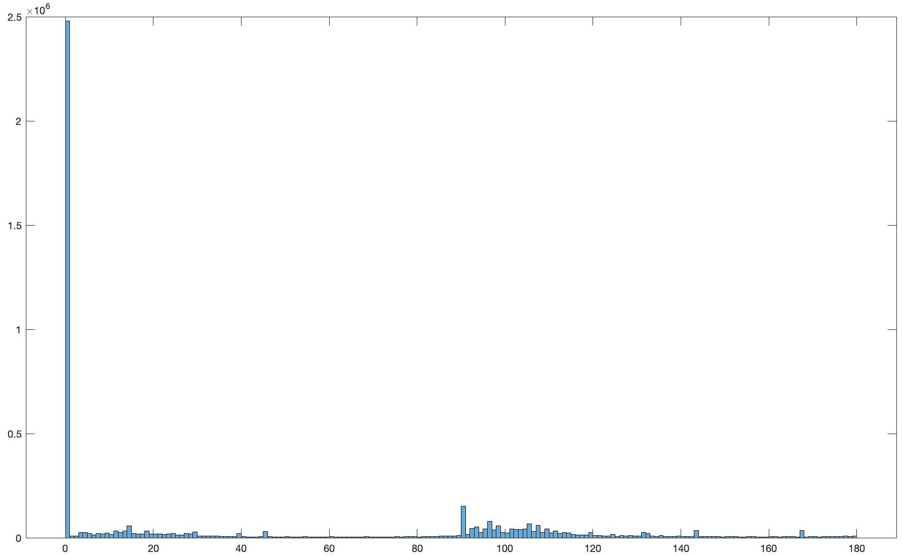
As we mentioned before, a large area with same color might influence the straighthening result unpredictably. For this example, the input above has few lines in it, and the edge plot shows few white lines while most of the pixels are being just black. Those black pixels dominate and have unpredictable influences on the angle distribution.

.
.
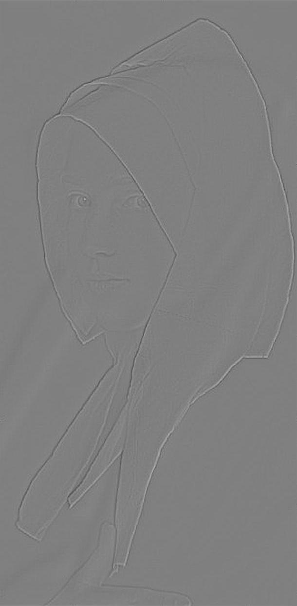
3 Image Sharpening (high frequency filter)
In this part, instead of bluring an image, we are going to use Gaussian filter to sharpen an image. If we subtract the filtered image from original image, the part with highest frequencies (sharpest part) will be left. By adding this sharpest part back to the image, we can gain an a sharpened image.

3.1 Blur then Sharpen
If we blur an image using a Gaussian filter first then try to recover it using sharpening method mentioned before, we notice that there is still some information lost during the process.
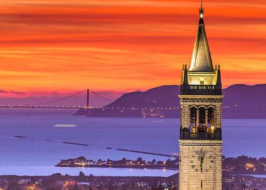
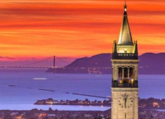
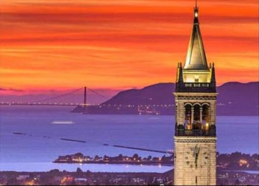
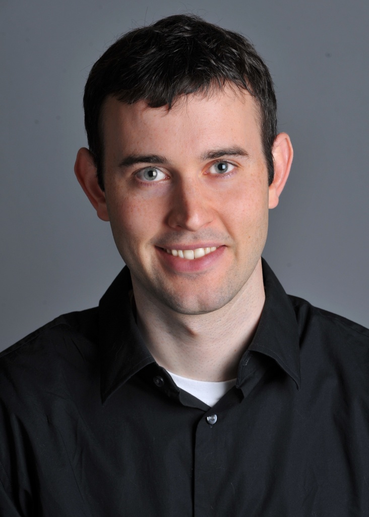
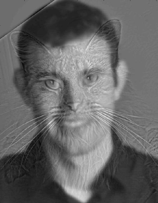
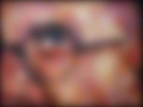
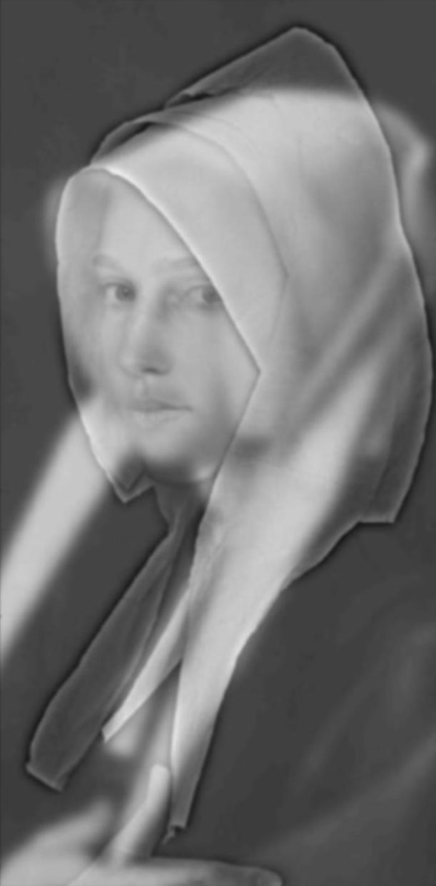
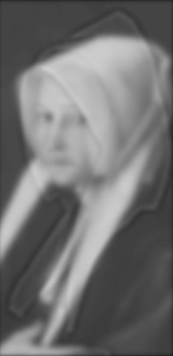
4 Hybrid Image (combined high & low frequency filters)
By combining high frequency filtered image and another low frequency filtered image, we can produce an hybrid image which will show high-frequency image when audience is close to the screen and loww-frequency image when audience is far away.

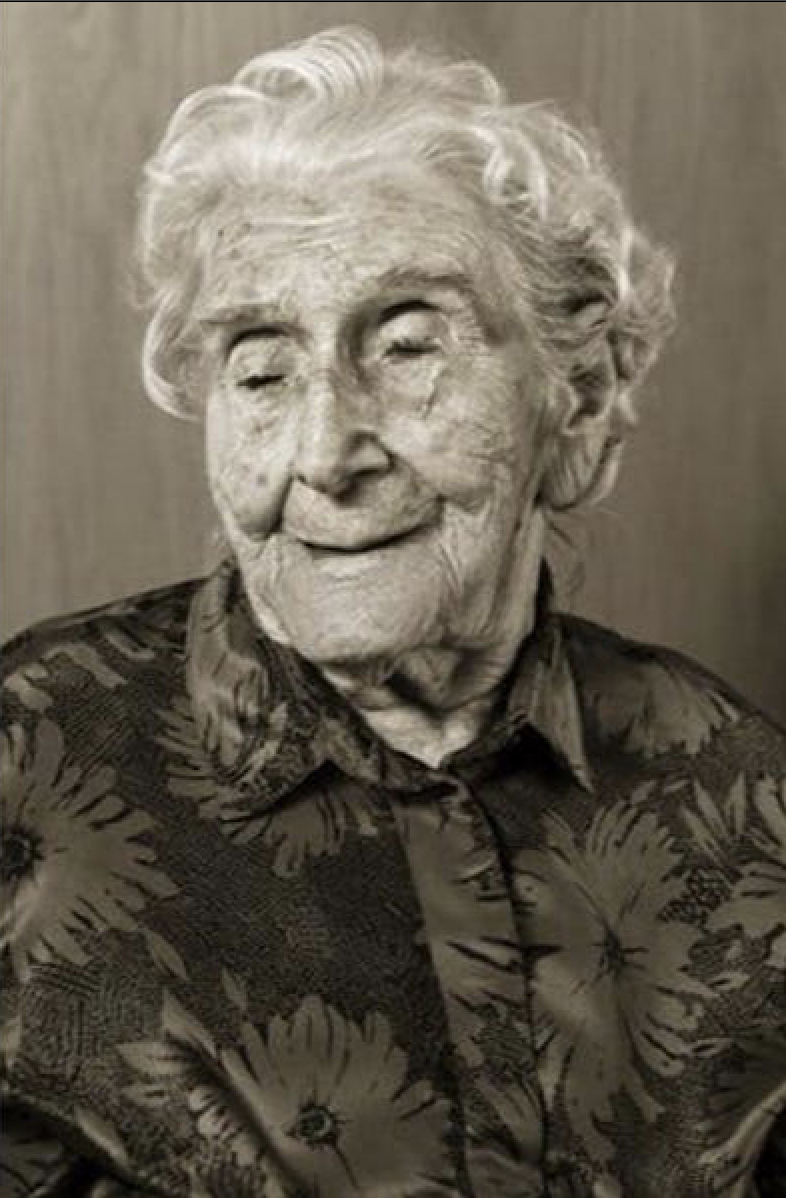
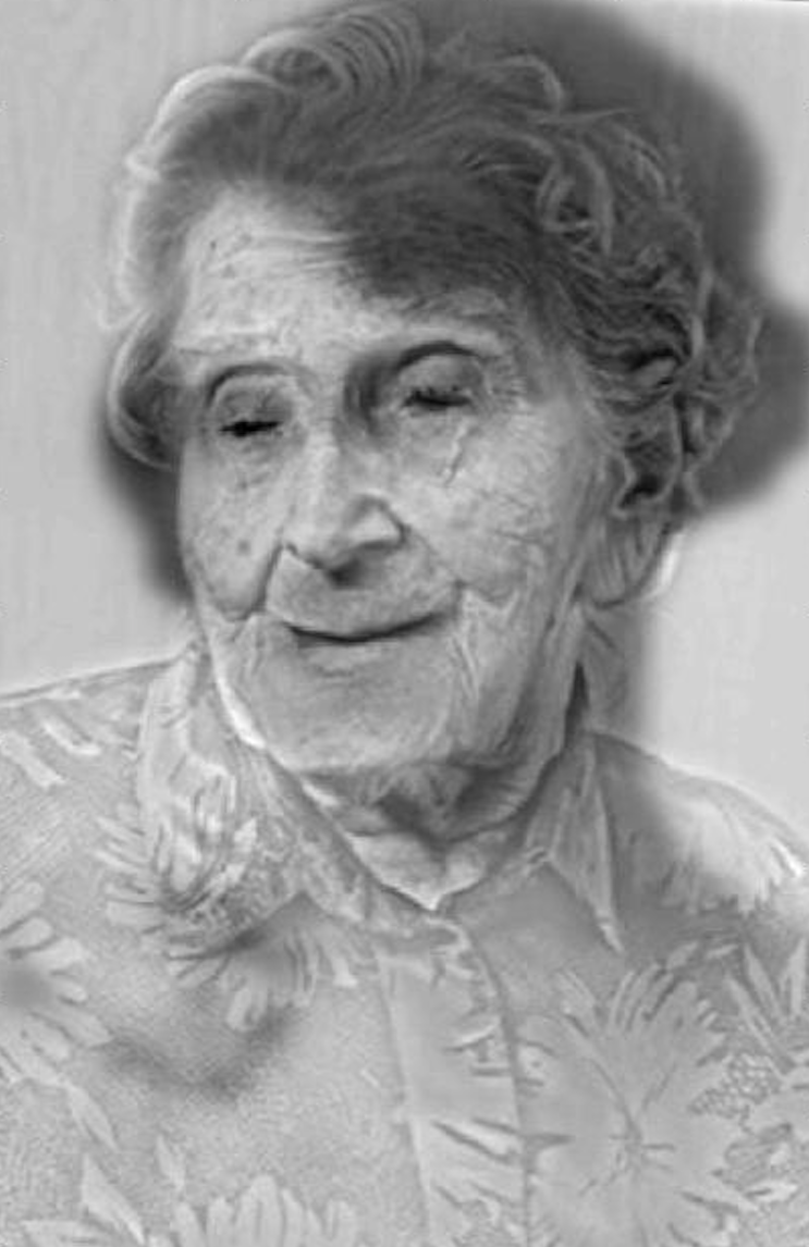
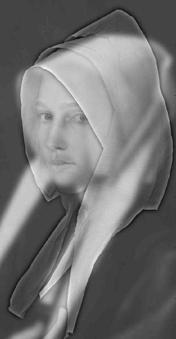
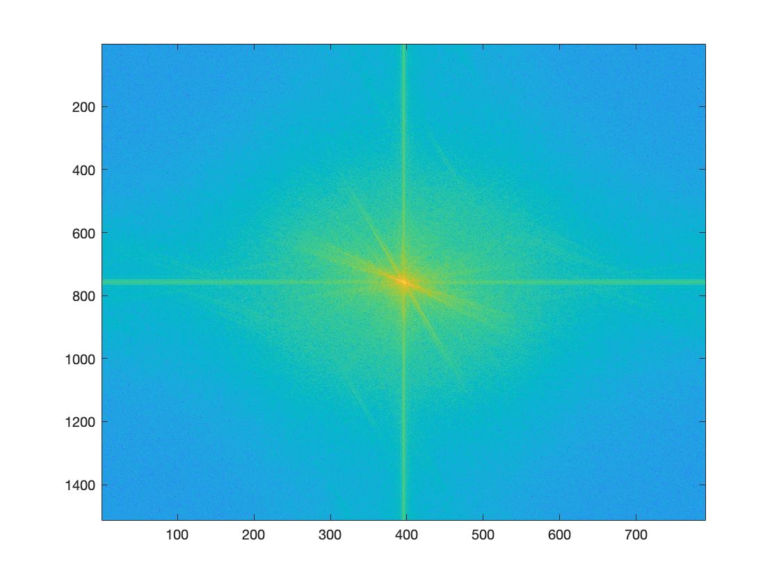
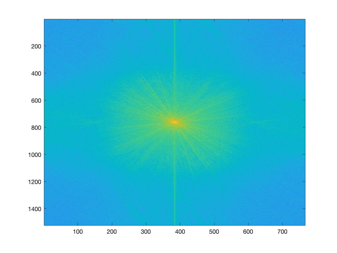
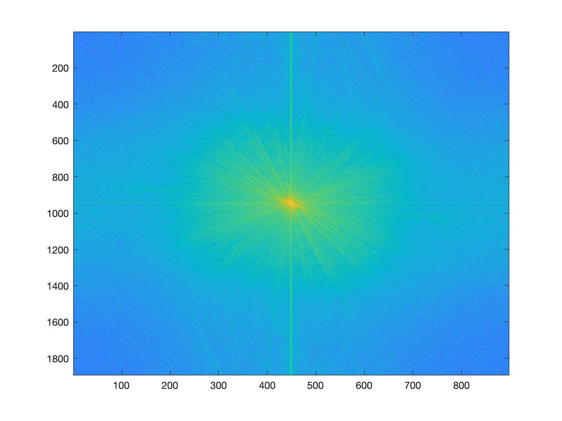
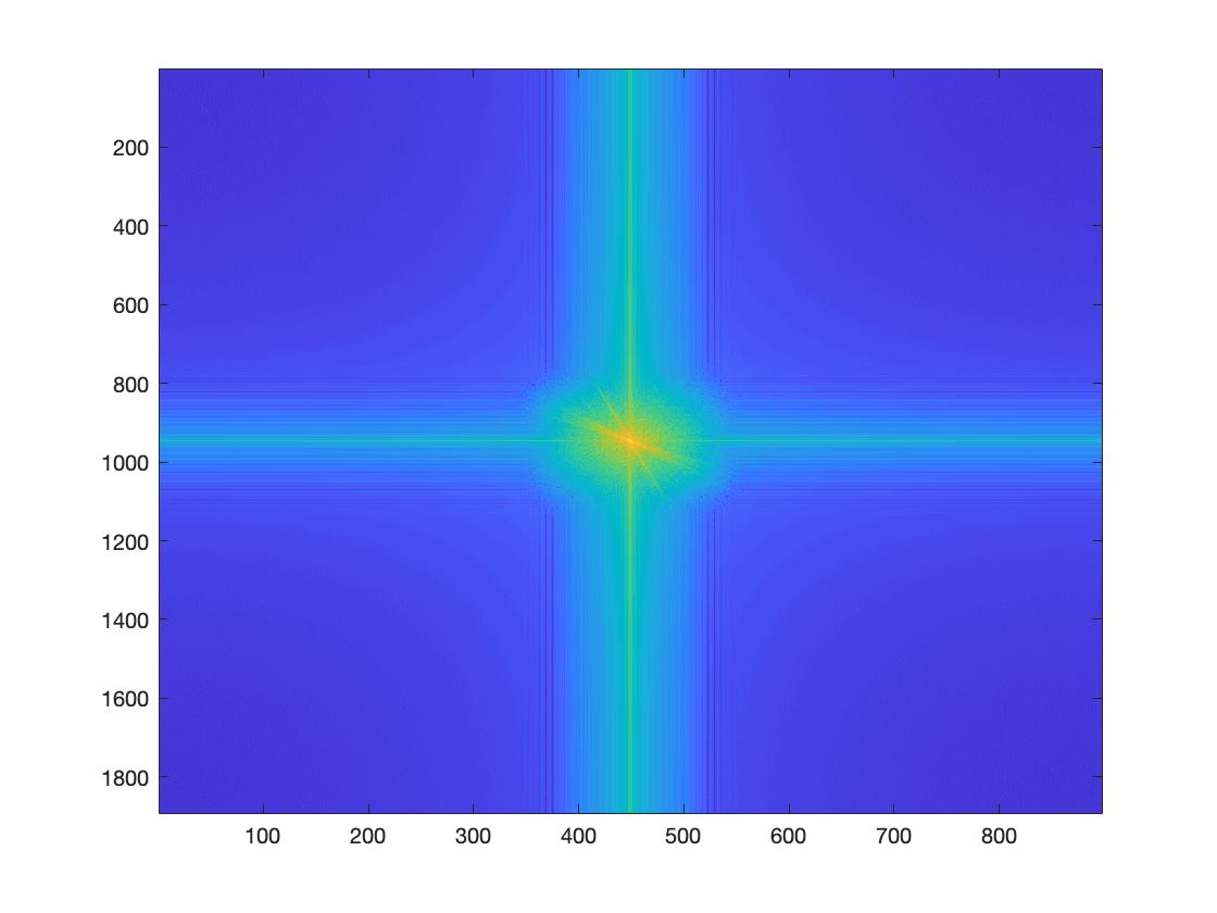
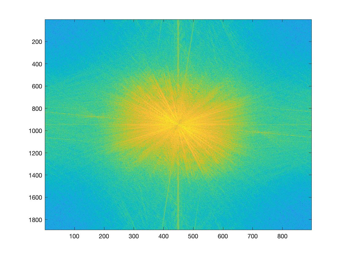
For next example, we are going to do frequency analysis. As we can see, although the frequencies of the two input images are similar, only low frequencies are left for filtered input 1 and only high frequencies are left for filtered input 2. Tshere is no ringing effect on the result frequency plot, which means the result image is smooth.


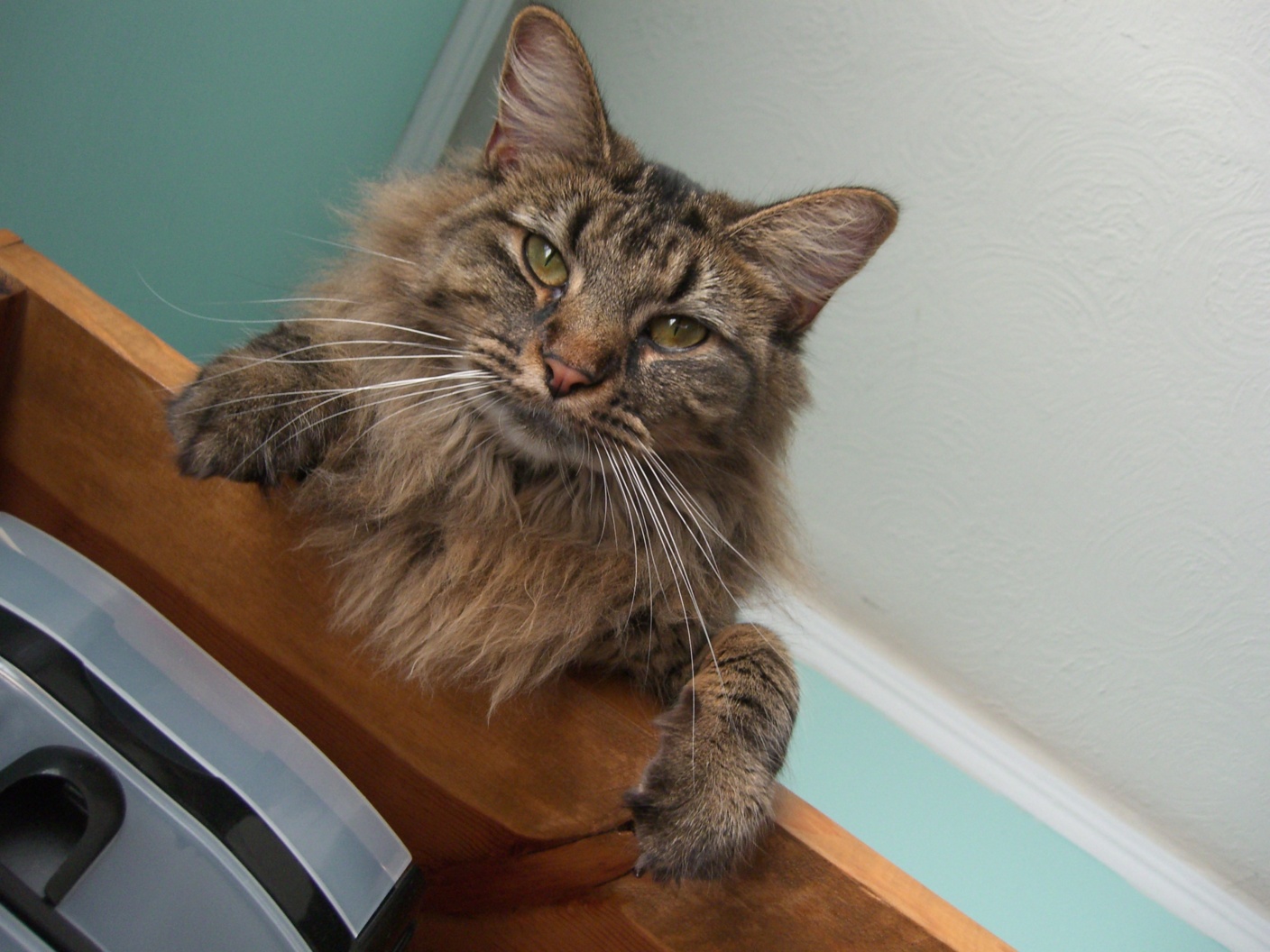
Failure Case:
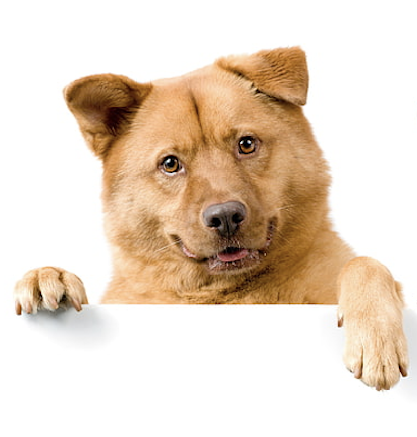
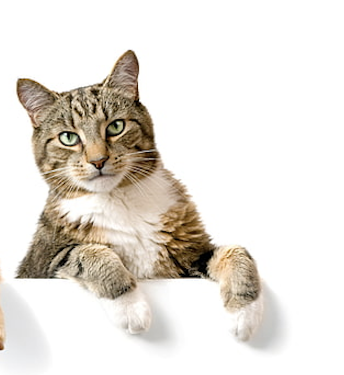
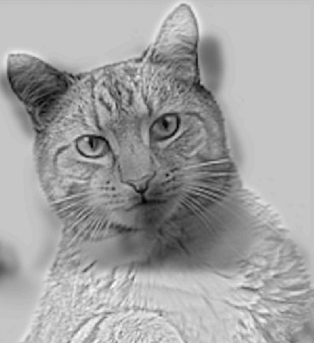
In the following example, because the cat in the second image has overall more black tone compared
to the dog in the first image, its high-frequency filtered result has strong and clear edges which
dominate the hybrid image over the very blurred dog image. Therefore, even if we stay far away from the
hybrid image, we may still only see the cat instead of the low-frequency dog.
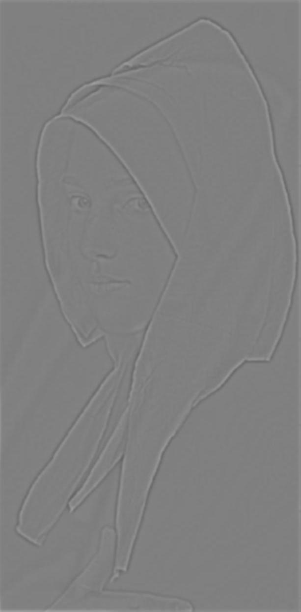
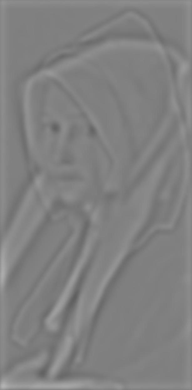
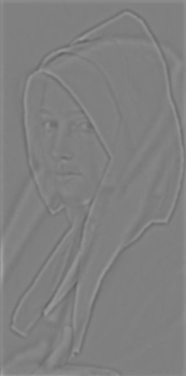
5 Gaussian and Laplacian Stacks
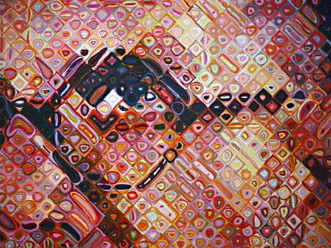
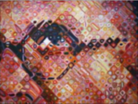
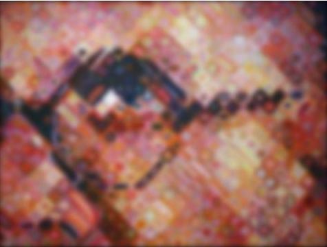
Now we want to look at Gaussian stacks with increasing sigma for Gaussian filters and corresponding Laplacian stacks. For Gaussian layer 1, 2, 3 and 4, the sigmas for the Gaussian filters are 2, 2^2, 2^3, 2^4 reqpectively. Laplacian layers are calculated by subtracting the Gaussian layer in the same level from the Gaussian layer in the previous level. Higher the level, lower the frequency that the Laplacian layer contains. Here we have examples of an interesting painting as well as the hybrid image we created in last section.


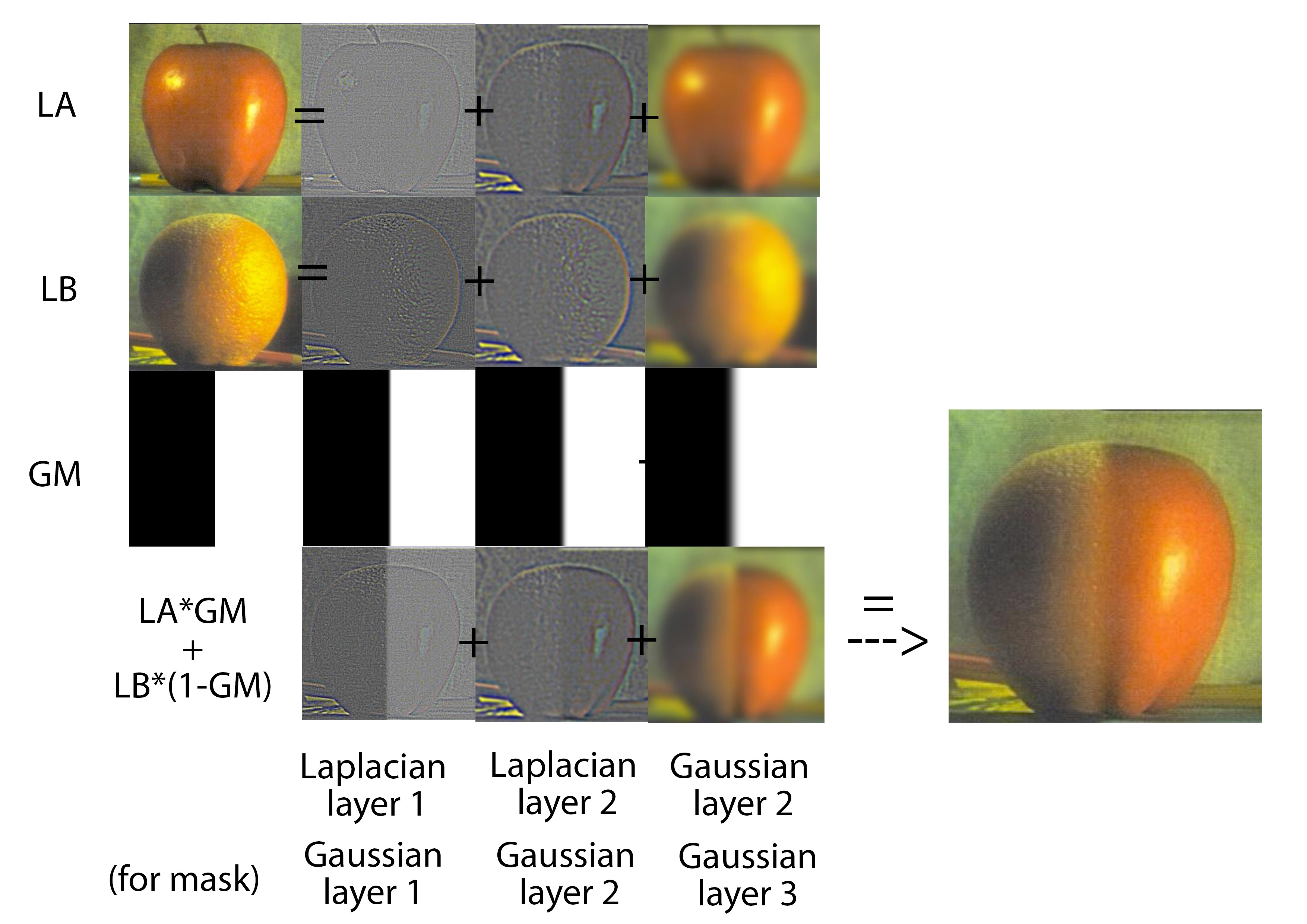
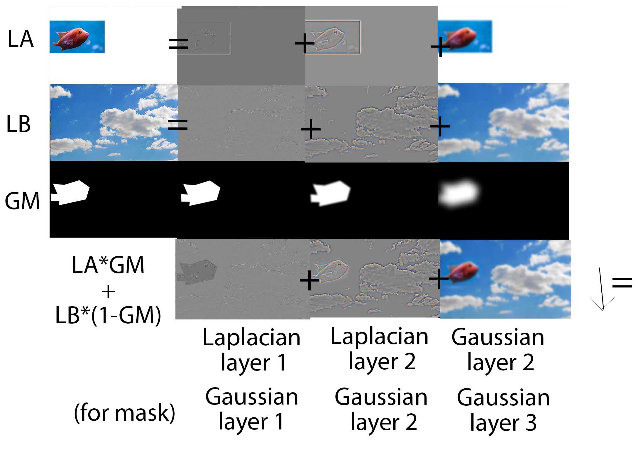
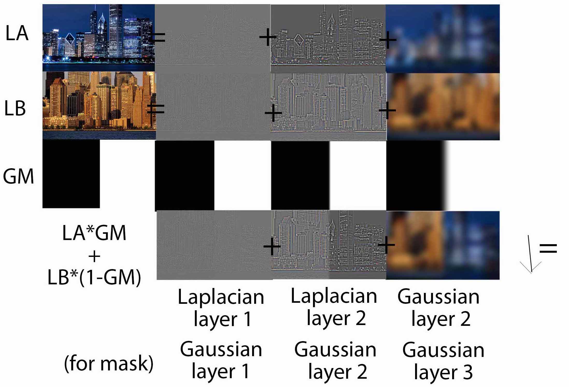
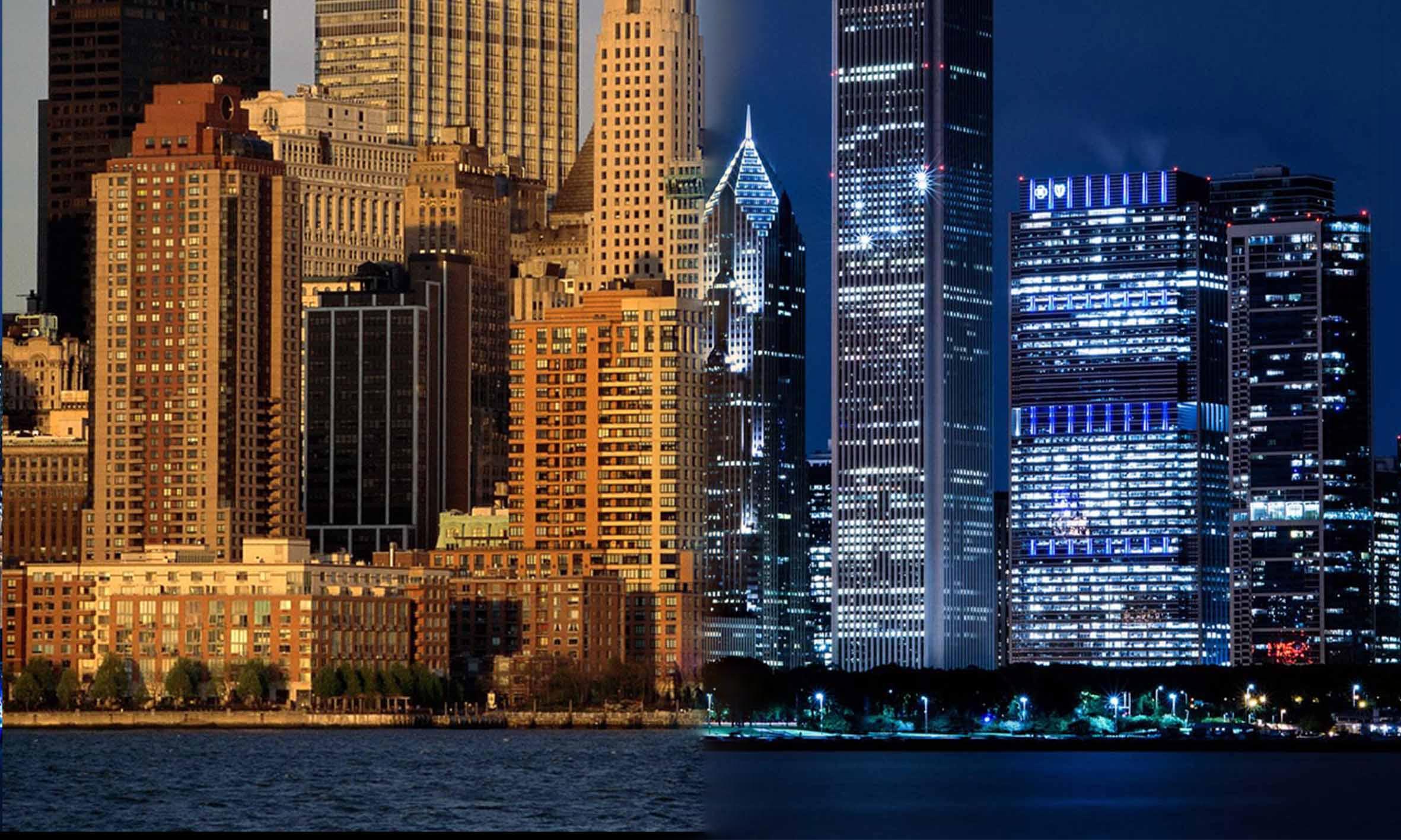
6 Multi-resolution Blending
Now we are ready to blend two iamges together smoothly using Gaussian and Laplacian stacks! Instead of just put half
and half iamges together and having a clear boundary between the images, we separate each image into Laplacian
layers and one final Gaussian layer (so the sum of all these layers will be the original image) to better blend the
two images. The Laplacian stacks make sure we preserve details and clear edges, while the base Gaussian layer makes
the blending smooth and looks natural. We also use Gaussian stacks for masks. The second step is to
apply masks onto images in every layer using LA*GM + LB*(1-GM), where LA is Laplacian layer for image A, LB is
Laplacian layer for image B, GM is Gaussian layer for mask, and teh result is a combined image for that layer (last
row on the graph). The last step is to add up combined images for all layers (don't forget last layer, which is
Gaussian stack for both images!).

7 Conclusion
In this project, we explored many interesting photo filters, and actually all these functions are achieved based on
convolution and Gaussian filters! The main idea is preserving/strengthening details using high frequency
filter (original image - gaussian filtered image) and reduce rapid random noise using low frequency filter
(gaussian filter). What I learned most from the project is that instead of manipulating the image directly, it will
always be beneficial to consider the image as a compound of low frequency part and high frequency part and then
deal with the two parts respectively according to their properties.
Photo source:
Section 4 young & old woman: https://www.thisiscolossal.com/2020/04/covid-19-getty-recreations/
Section 4 girl & painting: https://www.insider.com/young-vs-old-photo-portrait-comparison-100-years-2019-11
Section 5 painting: https://www.pinterest.com/pin/191966002836217780/