
|
|
|
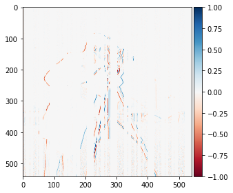
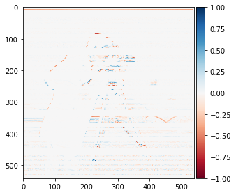
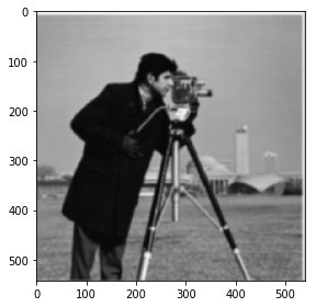
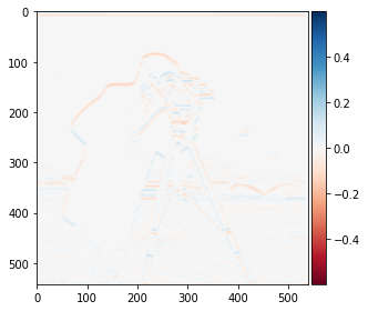
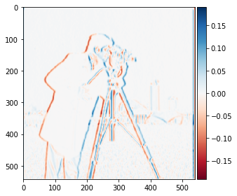
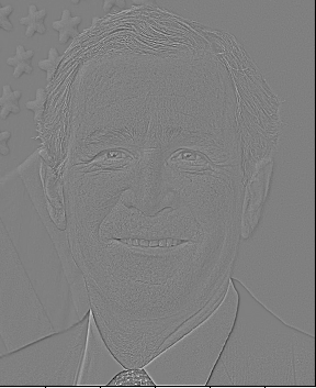
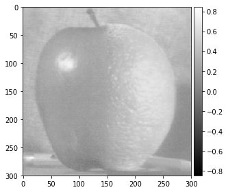
The goal of this section is to compute an image gradient. Since an image is a discrete form of data, we use the finite difference method to estimate the partial derivatives of the image in x and y. These partial derivatives immediately yield the gradient. The finite difference can be formulated as a convolution operation where convolution of the image with the row vector Dx = [1, -1] gives the x-partial derivative and convolution with the column vector Dy = [1, -1]. We apply these operations on the example cameraman image.
|
|
|
|
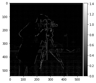
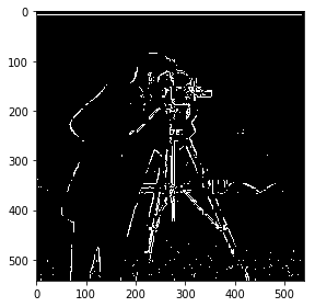
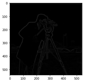
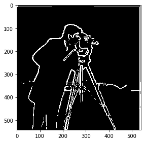
Adding the partial derivative images elementwise in quadrature, we obtain a gradient image which encodes the magnitude of the gradient in the image. By threshholding the magnitude of the gradient image, we create an edge detector
|
|
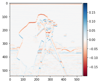
The result of the edge detection was noisy (notice the speckles at the bottom) without any preprocessing. We can remedy this by first applying a Gaussian filter to get rid of high frequency noise before applying our edge detection algorithm
|

|
|
|
|
Since convolution is associative, we instead of filtering with the gaussian followed by the finite difference filter, we can instead convolve the image with a hybrid filter, formed by convolving the gaussian with the finite difference filter, the derivative of gaussian filter.
|
|

|

|
These images demonstrate the equivalence of the hybrid filter and the sequential application of the gaussian and finite difference filter
|
|
|
|
|
|
|
|
|
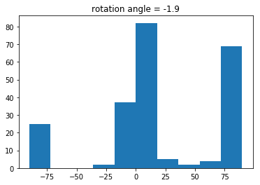
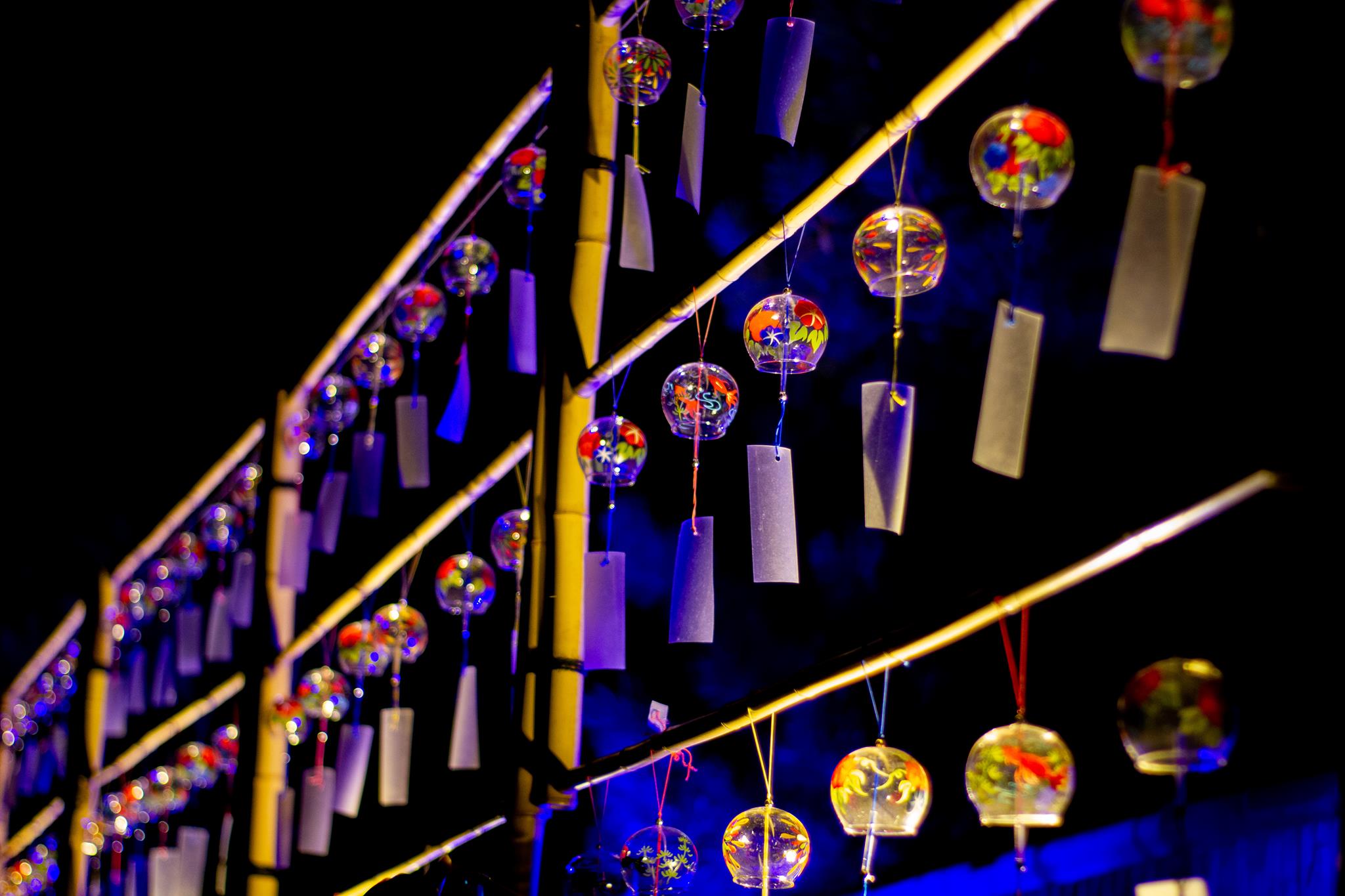
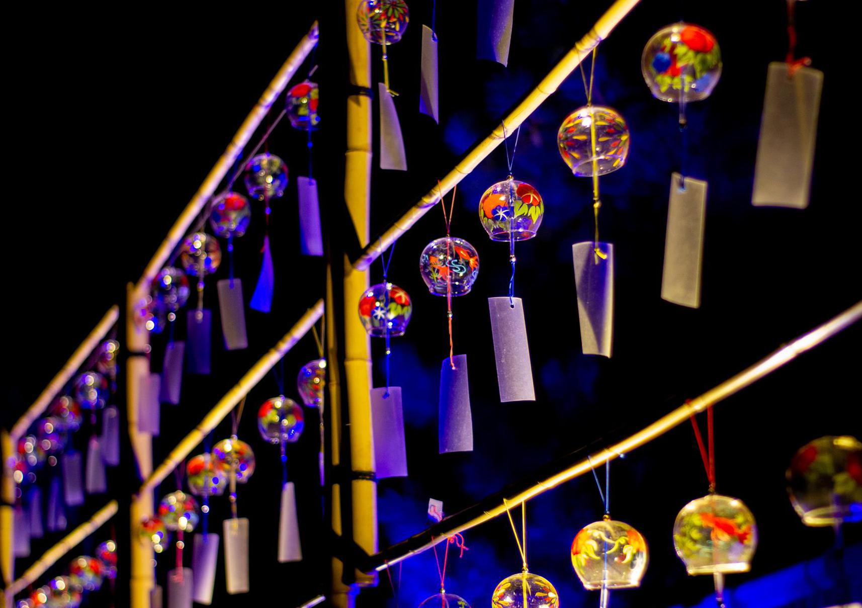
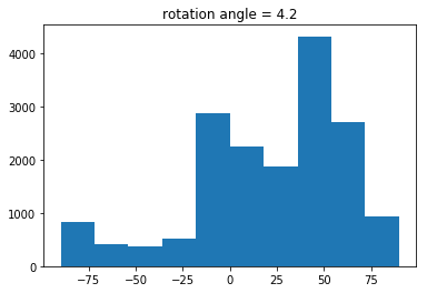
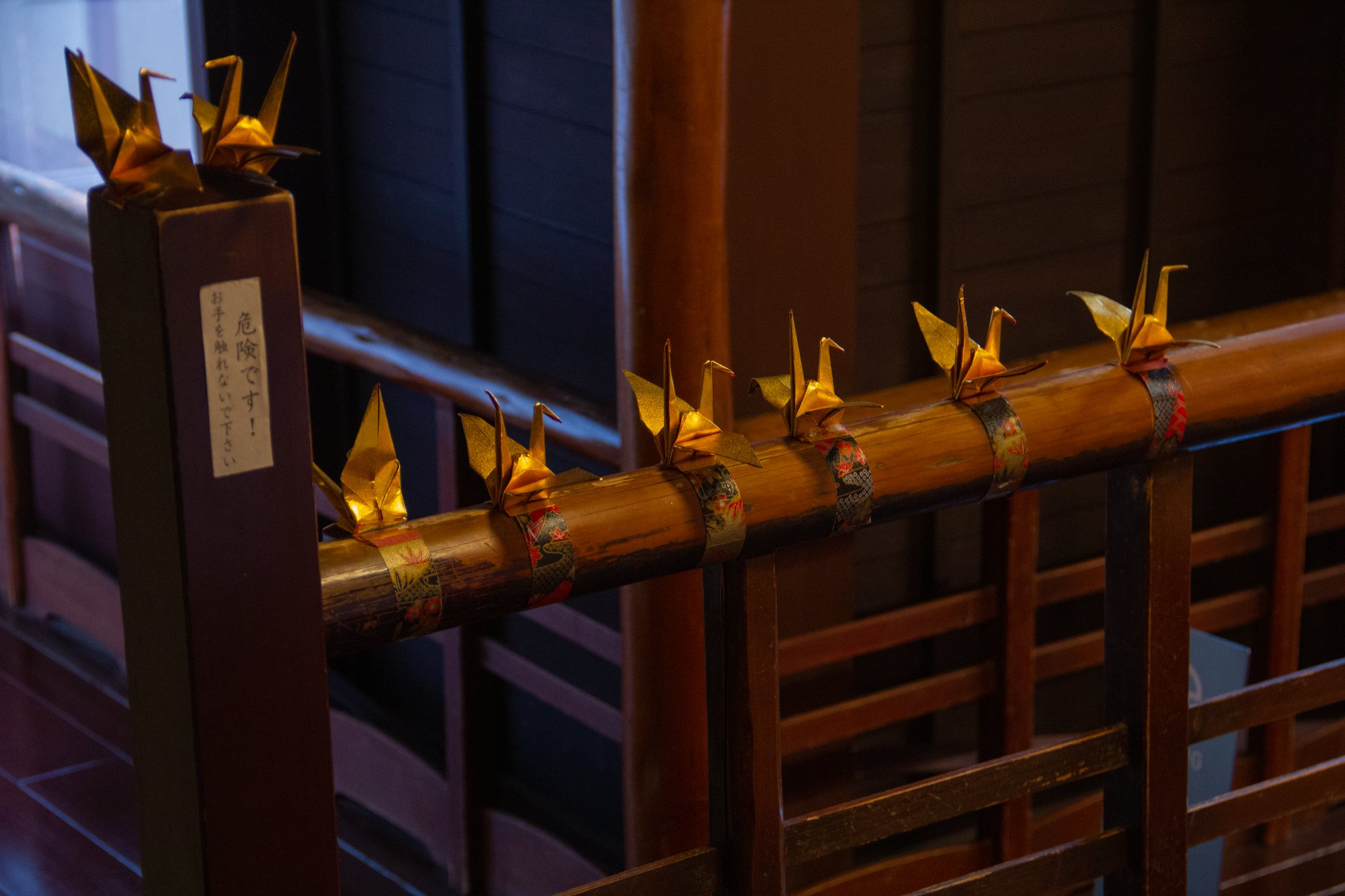
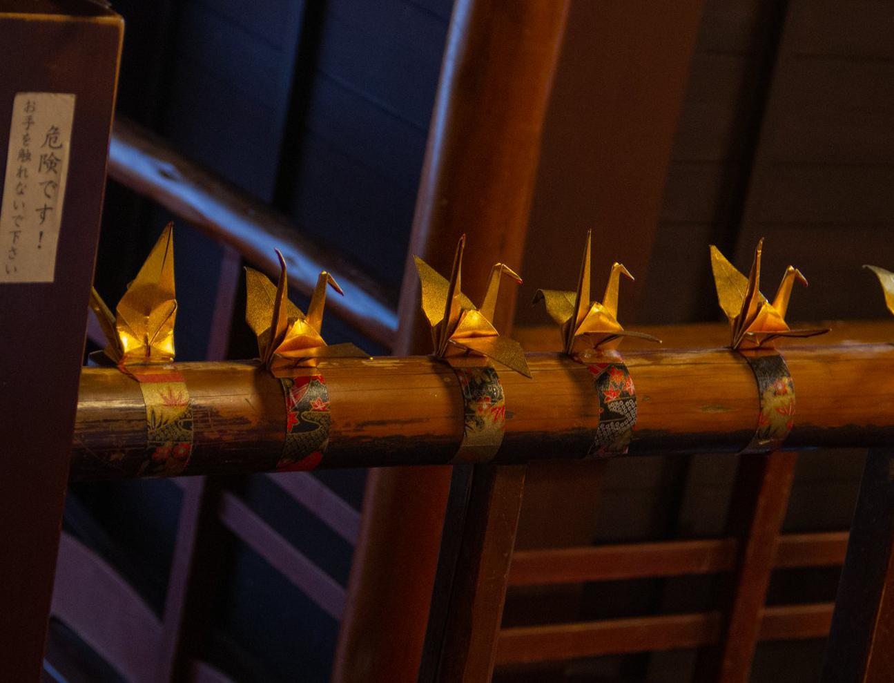
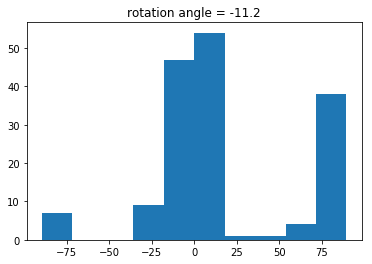
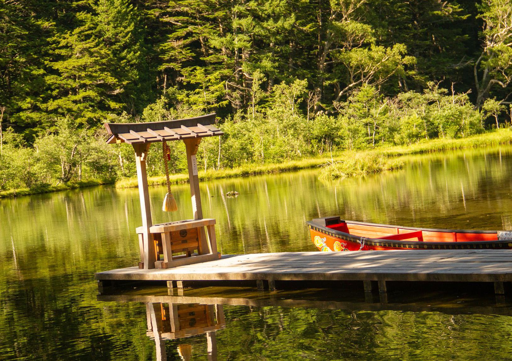
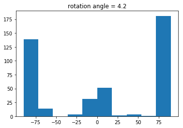
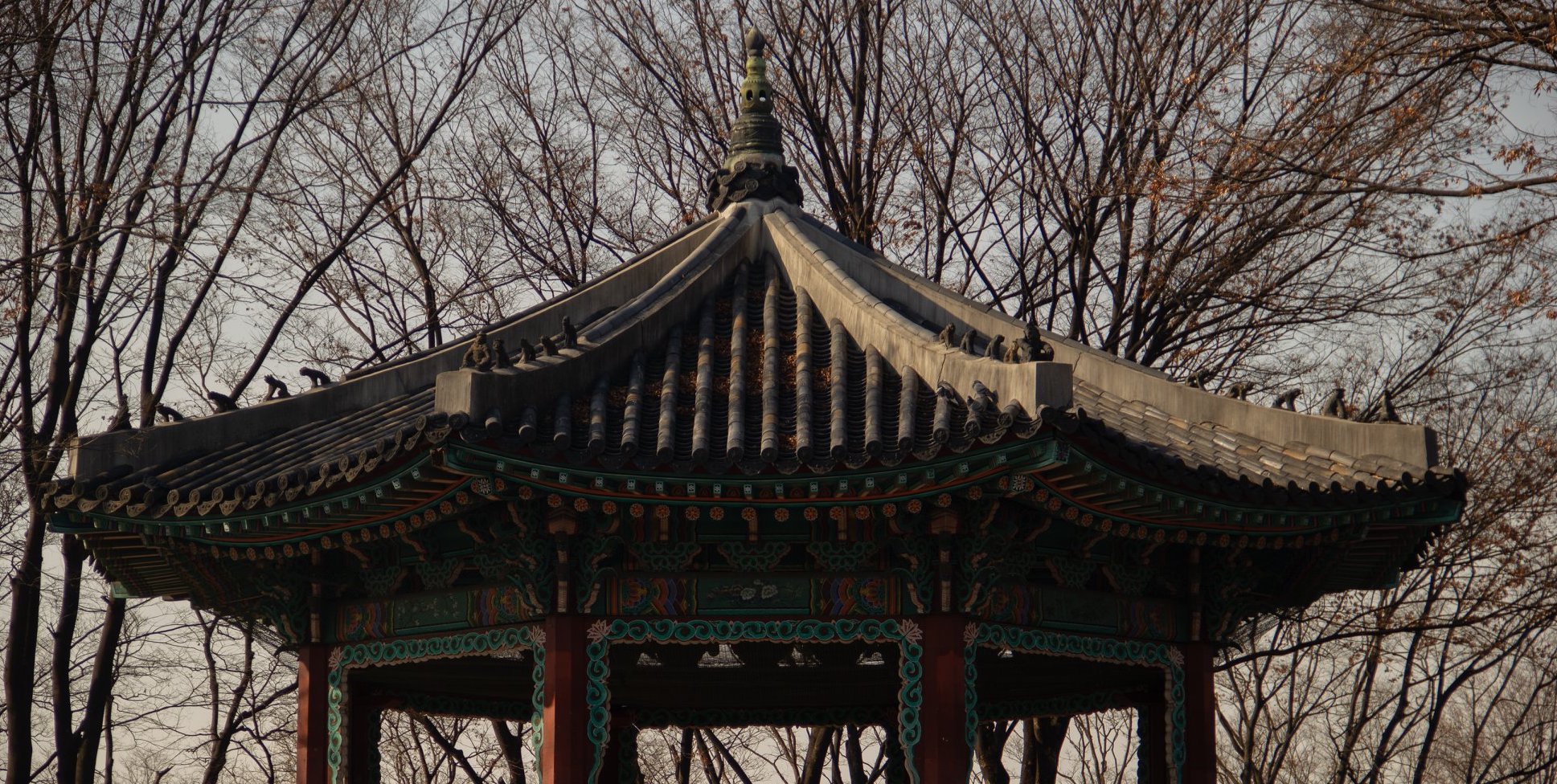
In the following image, the automated rotation fails. I attribute this to the fact that there is a long prominent edge (the boardwalk) that would dominate the edge count causing the rotation to try and make the boardwalk horizontally aligned rather than make the shrine vertical, which is shorter in length.
|
|
|
To create a sharpened image, we can extract the high frequency parts of an image and add them back to the original image. This creates an illusion that the high frequency components of the image are well captured and give edges more prominence. To get the high pass image, we subtract the original image against a blurred version and add this difference to the original image to sharpen.
|
|
We see that in the sharpened image that the lines formed from the tiling and textures appear darker in the sharpened taj.
|
|
|
|
|
|
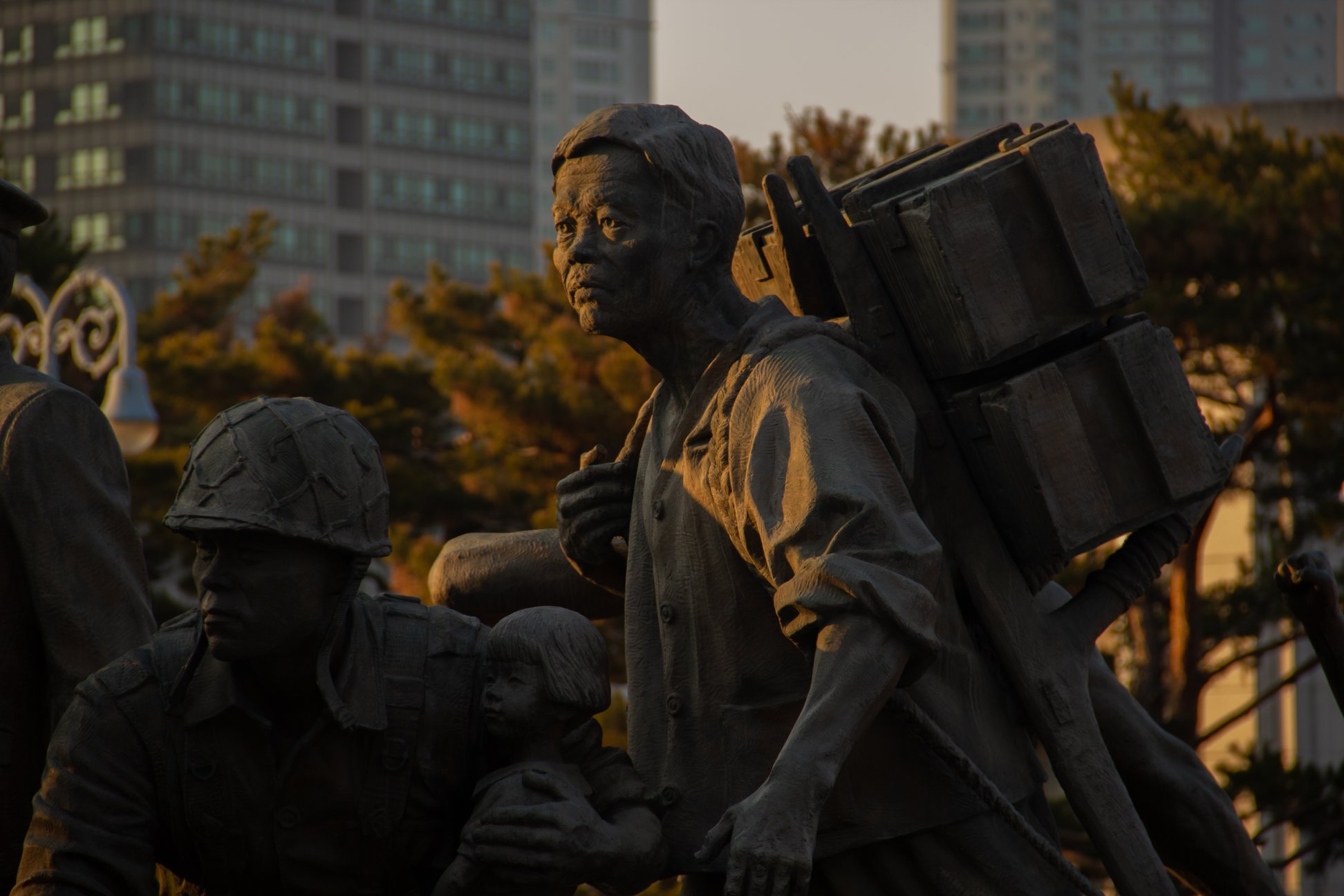
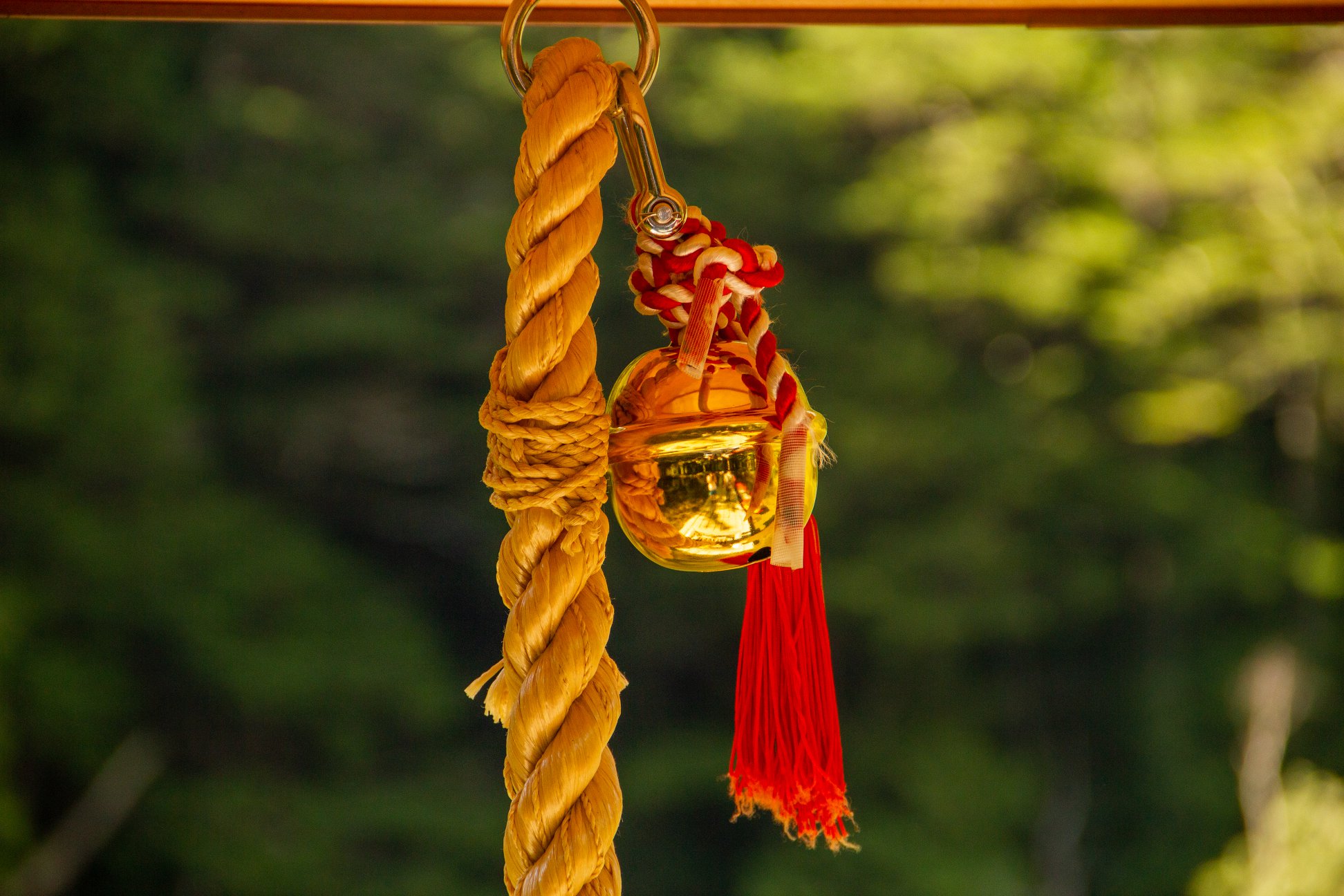
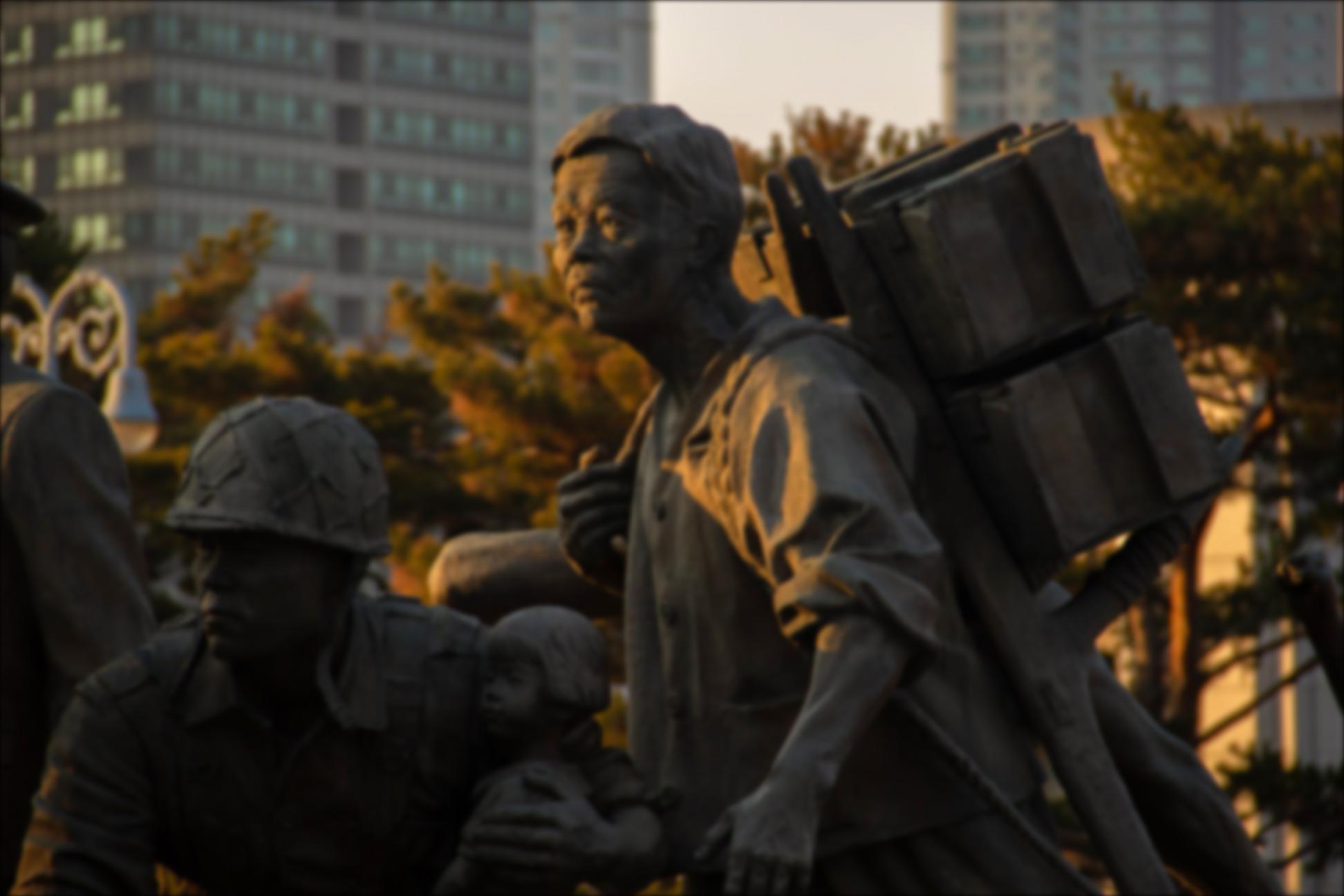
The effect of the sharpening can be seen to enchance the textures on the statue, the bell threads, and the tiling of the pagoda
Since sharpening doesn't add any additional information to an image, we cannot use it as a way to recover a blurred image. I illustrate this by attempting to blur and resharpen the statue photo.
|
|

|
|
Resharpening after blurring only returns a blurrier image than the source image
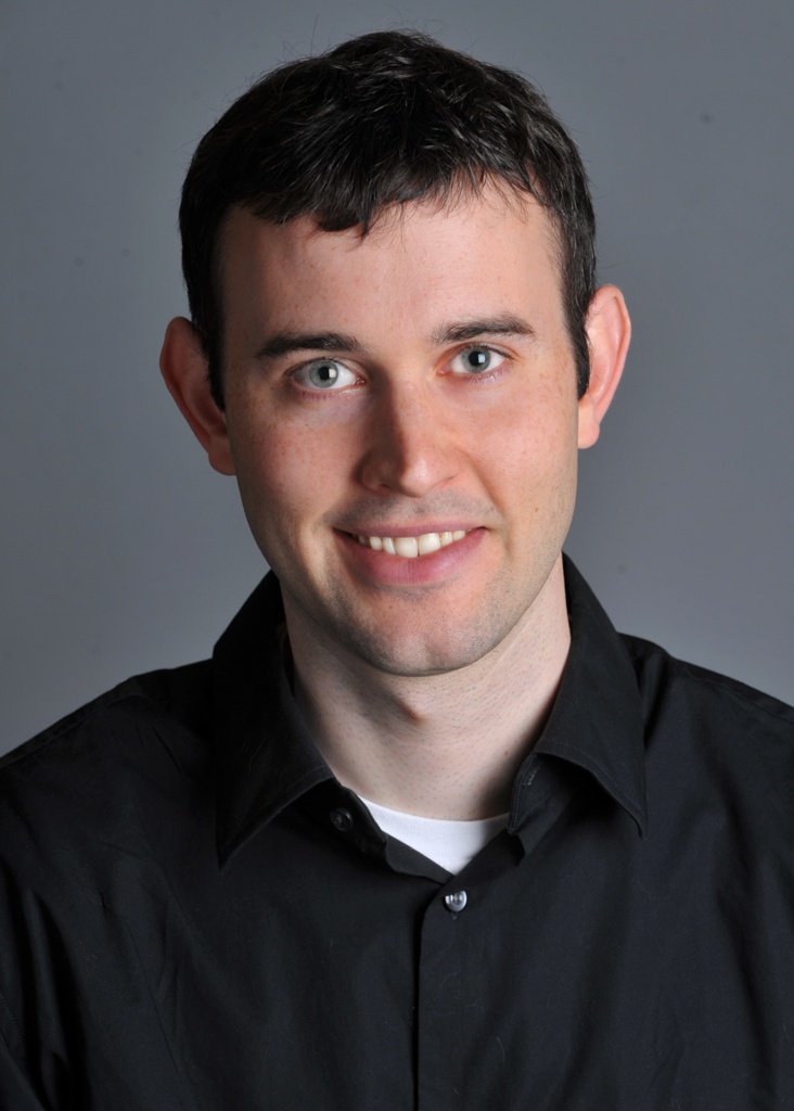
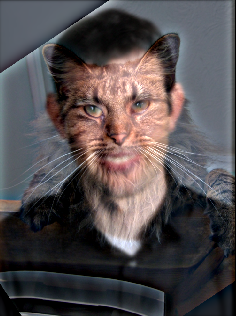
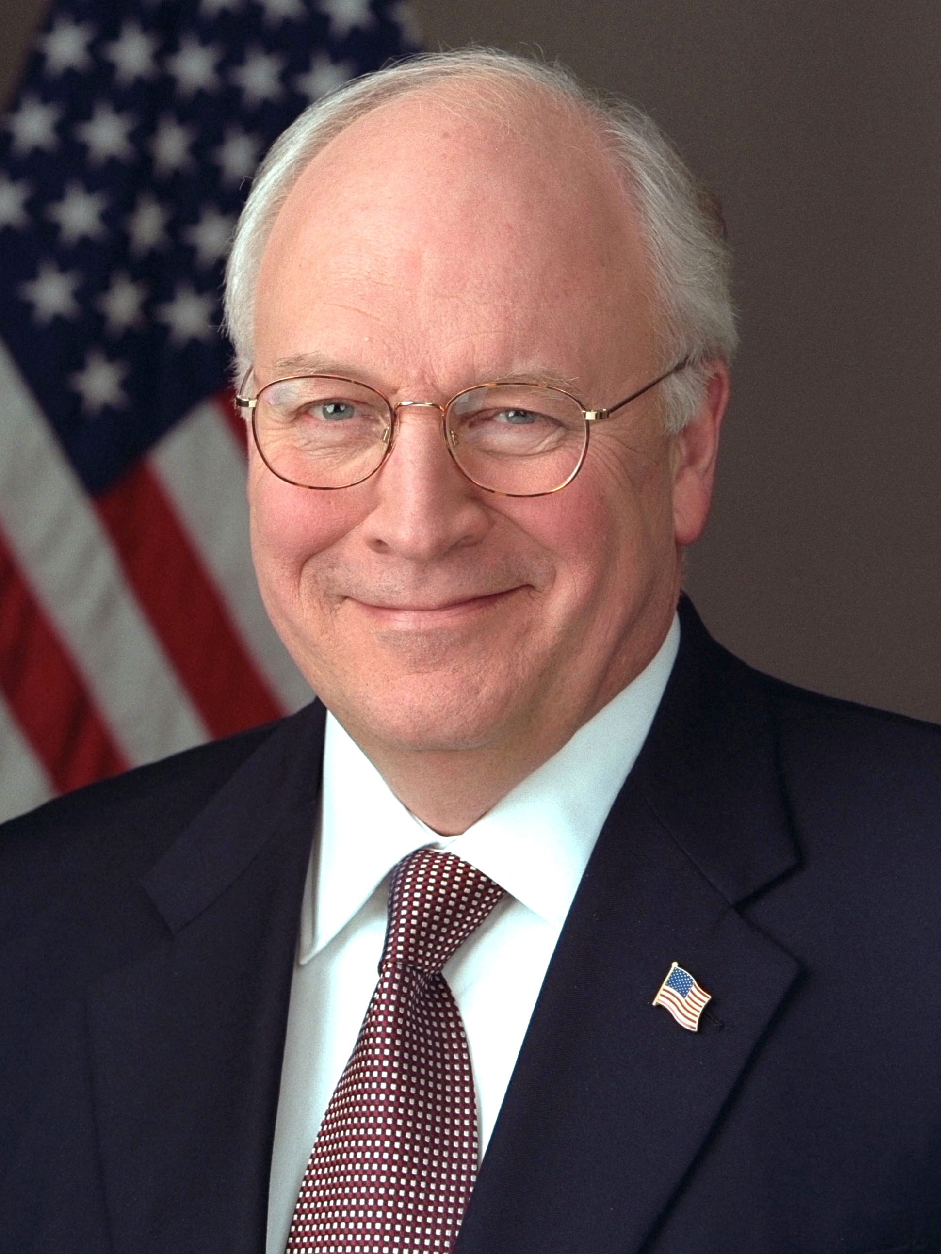
We can create a single image that changes intepretation with viewing distance by using two different images and adding the high frequency part of an image to the low frequency part of the other. The result is that high frequency component will be visible only at a short viewing distance while from far away, only the low frequency component is visible. To do this, we reuse our low pass and high pass filters from the previous sections to extract the bandpass images. Below are some results of this image hybridization.
|
|
|
|
|
|
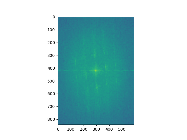
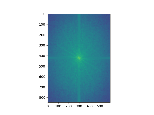
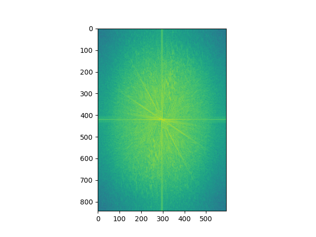
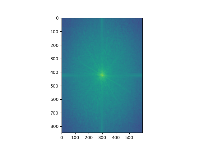
We can analyze each of the input images in fourier domain and see how the components when added frequency wise yield the final hybrid image.

|
|
|
|
|
|
|
|
|
|
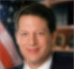
Evidently the final image is the composite of the high and low pass components as seen in the fourier domain. However, this hybrid image is not as compelling as the first two displayed due to the very different face structure of the two subjects. I believe the quality of the hybridization in for this pair of images suffers as a result
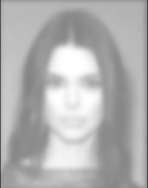
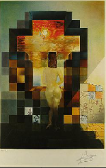
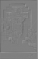
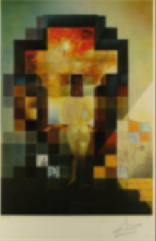
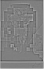
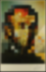
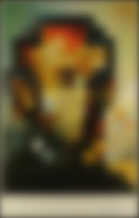
Using the our technique of high/low pass filtering, we can build Gaussian and Laplacian stacks. We can think of a Gaussian stack as a stack of images the encode information about a given image at different resolutions. For a Laplacian stack, each level just captures the difference between two successive Gaussian stack levels. We can use them to understand the structure of an image at different scales. Take for example the following Salvador Dali Lithograph of Lincoln after applying Gaussian/Laplacian stacks
|
|
|
|
|
|
|
|
|
|
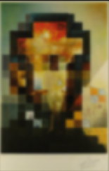
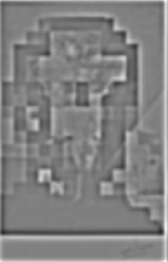
From the stacks we see that the structure of the Lincoln dominates mostly at lower resolutions while at the earliest levels of the stack we can see the microstructure within the lithograph
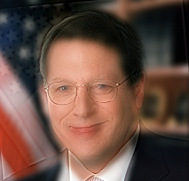
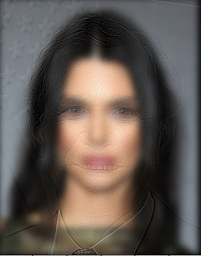
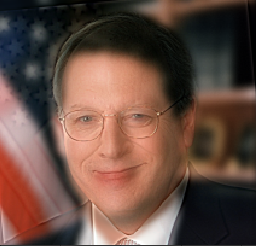
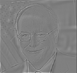
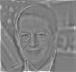
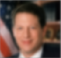
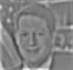
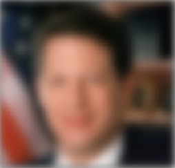
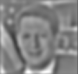
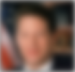
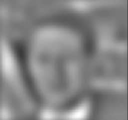
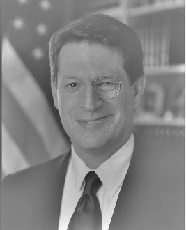
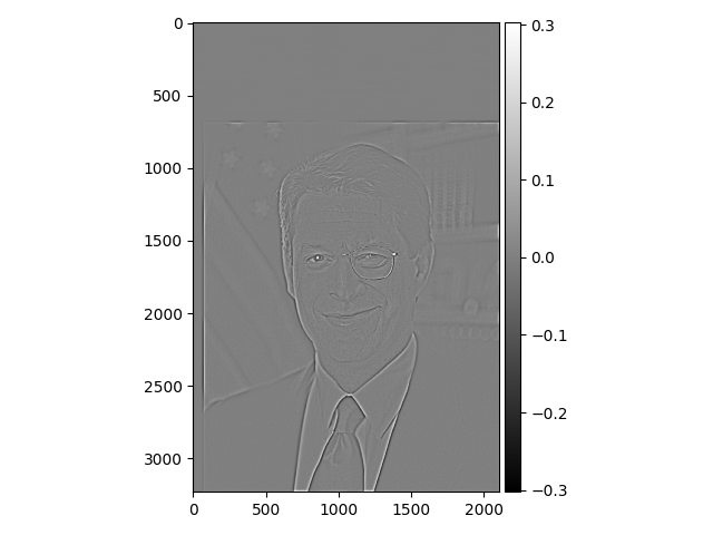
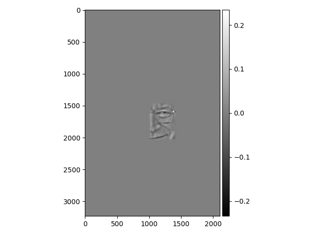
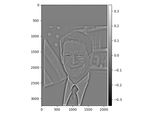
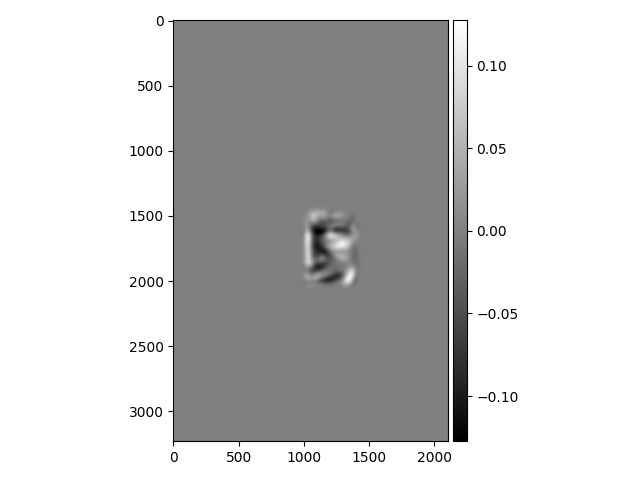
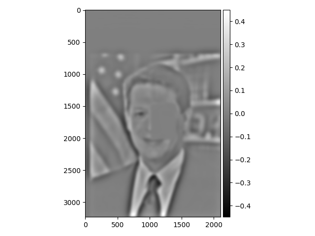
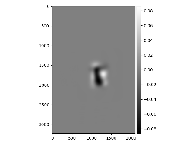
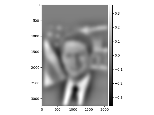
Let's use the laplacian stack to analyze the hybrid images we've made. The Algore-Cheney was our best result so we use it for this analysis
|
|
|
|
|
|
|
|
|
|
As we expect, the Cheney visage dominates at the earlier levels of the stacks whilst the Algore visage is more and more apparrent at lower resolution
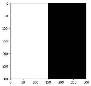
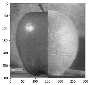
Using Gaussian and Laplacian stacks, we can blend two images together whilst reducing the seams creating by image stitching through multiresolution analysis. This works by creating laplacian stacks for our input images and a gaussian stack for our stitching mask. By adding together the levels of the laplacian stacks multiplied against the corresponding level of the stitching mask, we can produce smoothed blending boundaries. For instance, take this example apple and orange images.

|

|
|
|
|
|
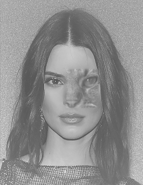
This technique doesn't only apply to vertical masks, we can make arbitrary masks for this technique and to good effect. Check out these face blends
|
|
|
|
|
|
|
|
We can analyze the blended gore-cheney image through our Laplacian stack to see how the image changes at each resolution level

|
|

|

|

|
|
|

|
|
|
|

|
|

|
|
Probably the most important thing I learned when debugging is making sure to increase my filter size when I'm increasing the sigma of the Gaussian filter. Also, I learned that using info at all resolution scales is necessary to successfully perform operations like image blending