CS194-26 Project 2: Fun with Filters and Frequencies!
Michael Park - Fall 2020
Objective
The main objective of this project is to explore different ways to use the Gaussian filter to produce interesting effects. A Gaussian filter can be applied to an image by convolving around it, producing a blurred effect. This can be used to separate different image frequencies and make blending images visually smoother. For this project, I made a step-by-step progression of tasks to familiarize myself with the Gaussian filter.
Finite Difference Operator
Before putting my hands on the Gaussian filter, I started with simpler filters. The goal of this
task was to convolve images with Dx = [1, -1] and
Dy = [[1], [-1]] filters, known as finite difference operators. First, I converted the
image to grayscale for simplicity. I used scipy.signal.convolve2d from the scipy
library to convolve the image according to Dx and Dy. Then, I performed a matrix-wise magnitude
operation to generate a gradient magnitude image.
I then generated a binary image, an image composed of only black and white colors, using an empirically determined threshold. I determined that setting the threshold at 0.225 was the best in my opinion. For the sake of comparison, I also generated a binary image using the Otsu's method.
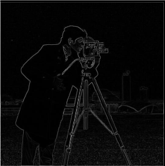
Below are the results for "cameraman":
Original

|
Gradient Magnitude Image
|
Binary with threshold=0.225

|
Binary with Otsu's Method

|
Derivative of Gaussian (DoG) Filter
Unfortunately, the previous method does not fully capture all visible edges. Also, its results are rather noisy, containing inconsistensies that should be ignored. To remedy this, a Gaussian filter can be used to reduce noise before processing.
To generate a Gaussian filter, I used cv2.getGaussianKernel to create a Gaussian
kernel. I set ksize = 11 and sig = 1 for this particular image. Since this
kernel is one-dimensional, I performed an outer product by itself to construct a 2D Gaussian filter.
Then, I convolved this filter around the input, and then performed the same operations as the
previous task. For this part, I set the empirical threshold to 0.095. Using the filter drastically
reduced the noise and captured more visible edges. As opposed to the previous set of images, the
edges of the cameraman in the current set of images are mostly connected.
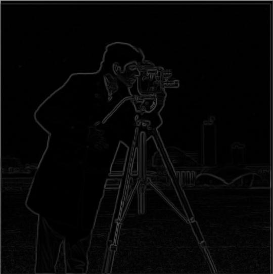
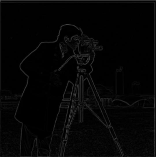
To verify that I performed the convolutions correctly, I attempted to perform the same operations by using a single step of convolution instead of two. This step was simple: before performing the operations, I found the derivatives of Gaussian by convolving finite difference operators around the Gaussian filter. Below are the results for "cameraman":
|
Original
|
Gradient Magnitude Image
|
Binary with threshold=0.095

|
Binary with Otsu's Method

|
Derivative of Gaussian (Dx)

|
Derivative of Gaussian (Dy)

|
Gradient Magnitude Image with DoG
|
Binary with DoG and threshold=0.095

|
Binary with DoG and Otsu's Method

|
Image Straightening
The main objective of this task is to automatically rotate an image to look straight. While there are no objectively correct ways to take a picture, there is a general consensus in preferences for vertical and horizontal edges in most images. To address this issue, I created a function that attempts to rotate an image so that the number of vertical and horizontal edges is maximized.
To simplify the process, my program attempts to find the optimal rotation angle over
[-10, 10) degrees. Detection of horizontal and vertical edges is not as simple as it
seems to be. First, I convolved the input according to finite difference operators. Then, I
generated a gradient angle matrix by finding the element-wise inverse tangent of
(df/dy) / (df/dx). To determine whether the edges are vertical or horizontal, I had to
check if the gradient angles are divisible by pi (given that these angles are in radians).
Unfortunately, not all angles fall into this category, meaning that not all edges are exactly
vertical or horizontal. To address this issue, I set bounds to the check so that angles can be
offset by 0.05 radian to qualify.
Rotating an image produces black outer spaces. This creates edges that should not be considered when calculating the gradient angle matrix. To address this issue, I used manual cropping so that only the center 60% of the images are considered.
This algorithm failed to find an optimal angle for some images. This is because the assumption that straight images have the maximum number of vertical and horizontal edges does not always hold true. For the Japan image, the crosswalk is not supposed to be perfectly horizontal. For the China image, topmost edges of the wall are hindering the image from correctly determining straightness. While this issue may be addressed by weighing vertical and horizontal edges differently, this may not work as well because our perception of straightness is not necessarily objective.
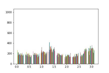
I also included the histograms of gradient angles of original images as well as rotated images for comparison. Below are the results:
Facade

|
Optimal Rotation: -3 deg

|
Original Histogram
|
Rotated Histogram

|
Korea

|
Optimal Rotation: 3 deg

|
Original Histogram

|
Rotated Histogram

|
Japan (Failed)

|
Optimal Rotation: 0 deg

|
Original Histogram

|
Rotated Histogram

|
China (Failed)

|
Optimal Rotation:: 0 deg

|
Original Histogram

|
Rotated Histogram

|
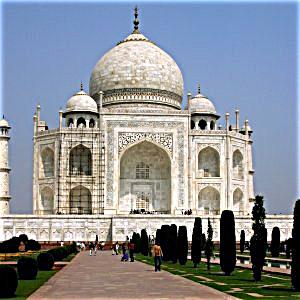
Image "Sharpening"
The Gaussian filter is considered a low pass filter that retains only the low frequencies of an image. This means that a high-frequency image can be obtained by subtracting a Gaussian filtered image from the original "impulse" image. Using these two filtered images, I am able to create a sharpened version of an image.
For this task, I set ksize = 11 and sig = 3 for all images. I went through
the same steps as before to create Gaussian filtered images. Then, I took the difference from
original images to generate high-frequency images. Lastly, I experimented with different alpha
values, or multipliers that determine how much of high-frequency parts will be accentuated, to
generate sharpened versions of images.
I tested with alphas = [1, 5, 10, 50]. Below are the results:
Taj

|
a = 0.5

|
a = 1
|
a = 5

|
a = 10

|
a = 50

|
Panda

|
a = 0.5

|
a = 1

|
a = 5

|
a = 10

|
a = 50

|
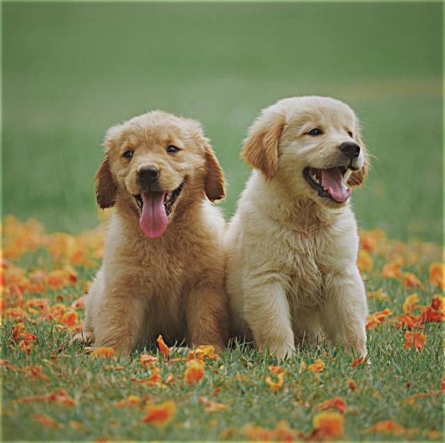
Dogs

|
a = 0.5

|
a = 1
|
a = 5

|
a = 10

|
a = 50

|
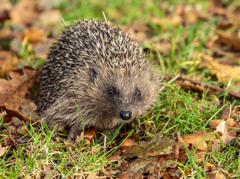
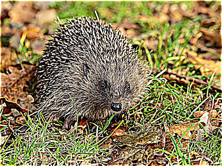
Hedgehog
|
a = 0.5

|
a = 1

|
a = 5
|
a = 10

|
a = 50

|
For evaluation, I took an image ("Taj"), blurred it using the Gaussian filter, then sharpened it again using the algorithm described above. While the image did seem to sharpen from its blurred state, I could not recover the original image from the blurred image. This is because the blurred image is missing the high-frequency parts that the original image initially had. Extracting high frequencies from the blurred image will not result in the same parts.
|
Original
|
Blurred

|
a = 0.5

|
a = 1

|
a = 5

|
a = 10

|
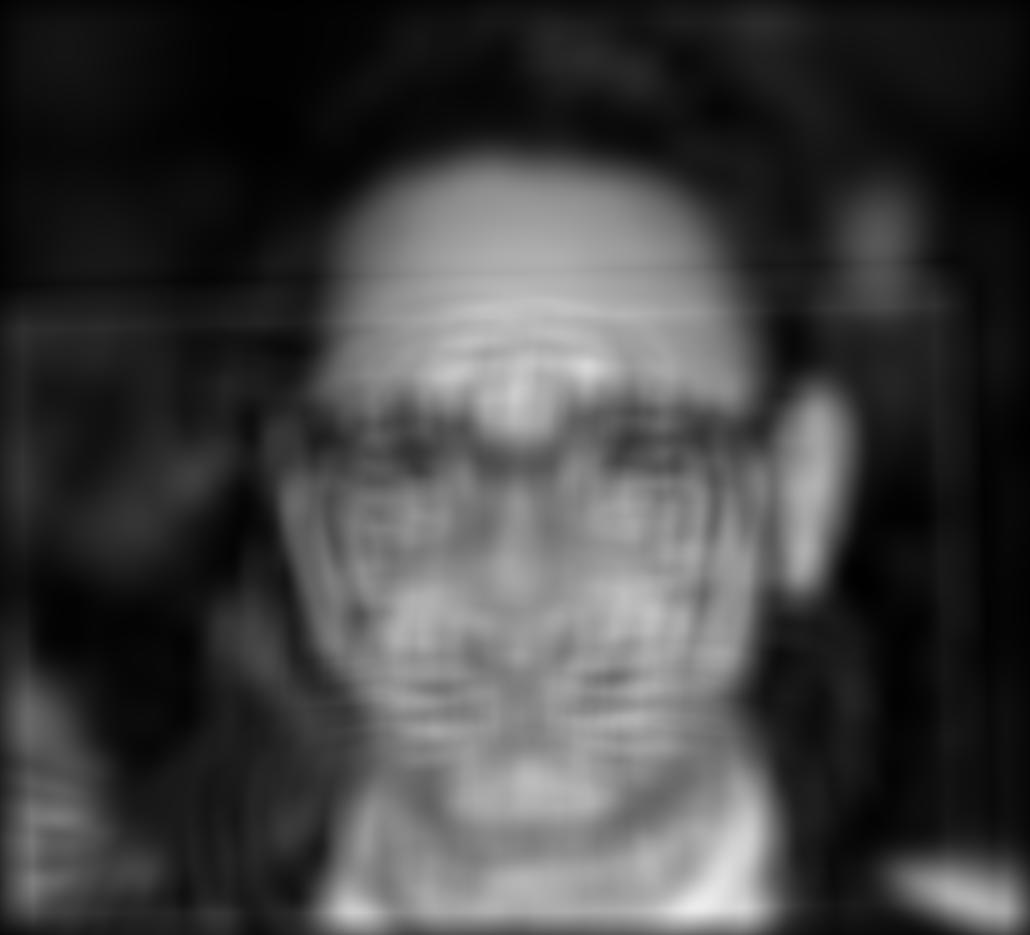
Hybrid Images
The previous task allowed me to separate high-frequency components from low-frequency components using the Gaussian filter. Using this, I can blend two images into a hybrid image, or static images that change in interpretation from different viewing distances. To create one, I need to extract high-frequency parts from one image, generate a low-frequency version of another, and then combine them together. While high-frequency image will be dominant from closer viewing distances, low-frequency image will start to show up from farther viewing distances.
After converting two images to grayscale, I first aligned them together by recentering, resizing,
and rotating. I generated two different Gaussian filters. For the low-pass filter, I set
ksize = 45 and sig = 5. For the high-pass filter, I set
ksize = 45 and sig = 100. Sigmas for the two filters are empirically
determined cutoff frequencies to filter out low and high frequencies, respectively.
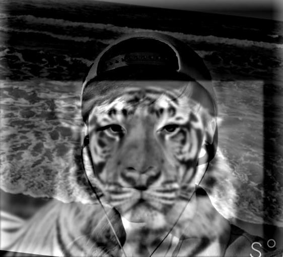
Notice that the last hybrid image does not fully reproduce the effect of a hybrid image. This is most likely because the tiger image has noticeably sharper features than the other. To mitigate this, I can set the cutoff frequency to be lower, but this may cause the tiger to be less noticeable. Below are the results:
Nutmeg

|
Derek

|
|
High Frequency

|
Low Frequency

|
Hybrid

|
Tiger

|
Robert

|
|
High Frequency

|
Low Frequency

|
Hybrid

|
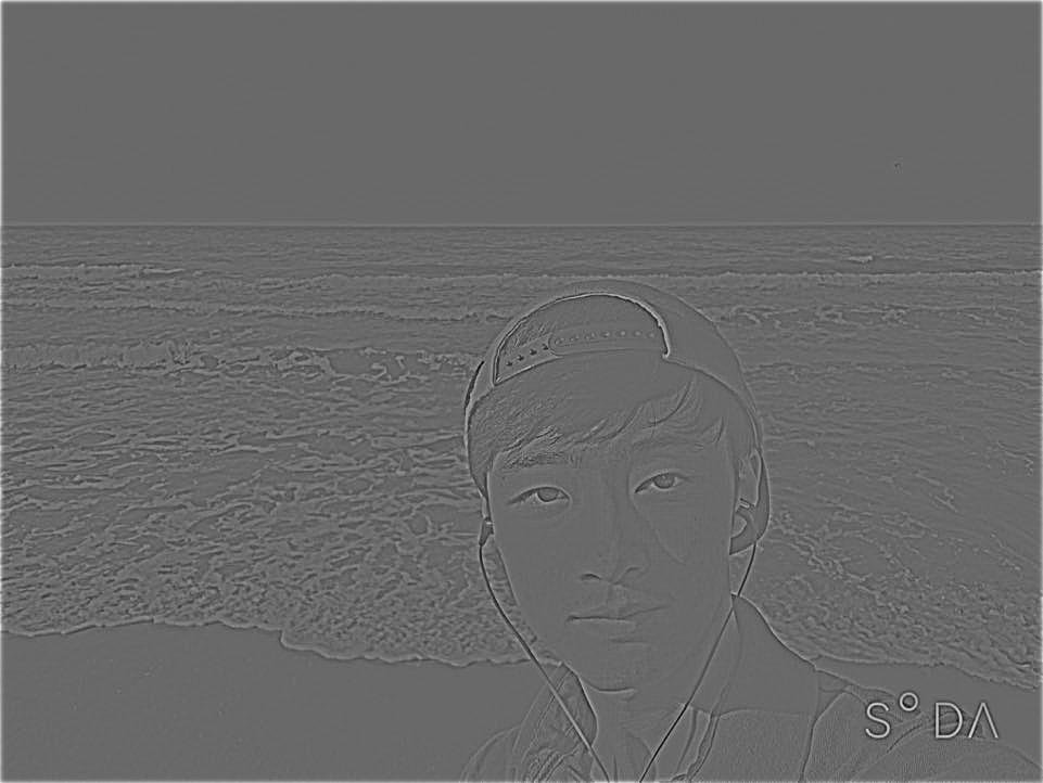
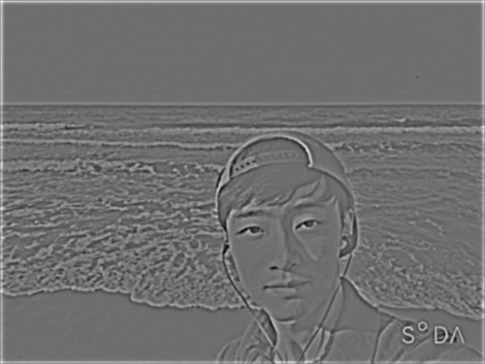
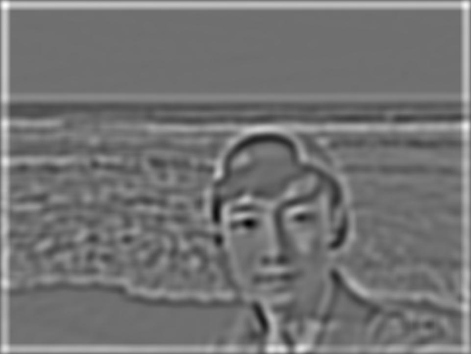
Denero

|
Sam

|
|
High Frequency

|
Low Frequency

|
Hybrid

|
|
Sam
|
Tiger
|
|
High Frequency

|
Low Frequency

|
Hybrid (Failed)
|
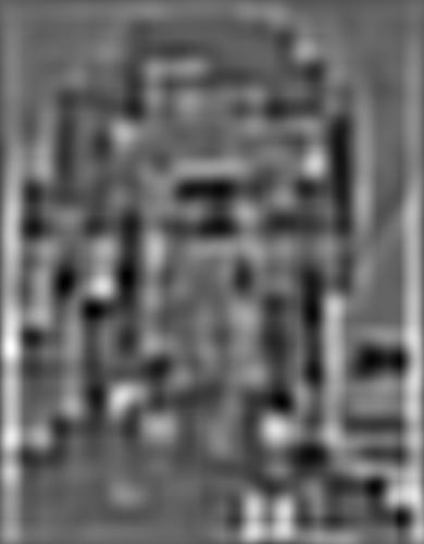
Gaussian and Laplacian Stacks
The main objective of this task is to implement Gaussian and Laplacian stacks. Gaussian stacks are layers of images that can be produced by convolving an image around Gaussian filters of different sigma levels. As sigma increases, the image becomes coarser, making it look blurry. In contrast, Laplacian stacks are layers of images produced by taking the difference between each layer of images in the Gaussian stack. This creates an interesting property: by summing up the images in the Laplacian stack and the last image in the Gaussian stack, I can reproduce the original image.
To create the Gaussian stack, I set ksize = 45 and sig = 2, 4, 8, 16, 32.
I followd thet same process as in previous steps to create Gaussian filters, and then convolved
around the original image. I subtracted the filtered images from images from the previous stack to
generate Laplacian stack images.
I defined my own imadjust function to make low-contrast images more visible. Below are
the results:
Lincoln
|
|
Gaussian 1

|
Laplacian 1

|
Gaussian 2
|
Laplacian 2

|
Gaussian 3
|
Laplacian 3

|
Gaussian 4

|
Laplacian 4
|
Gaussian 5

|
Laplacian 5

|
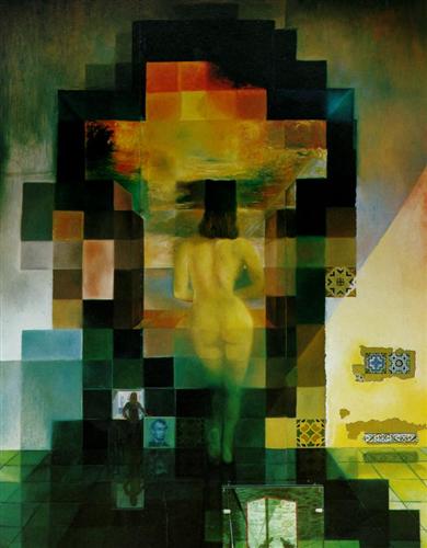
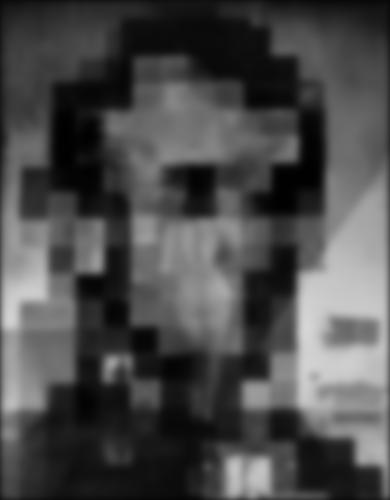
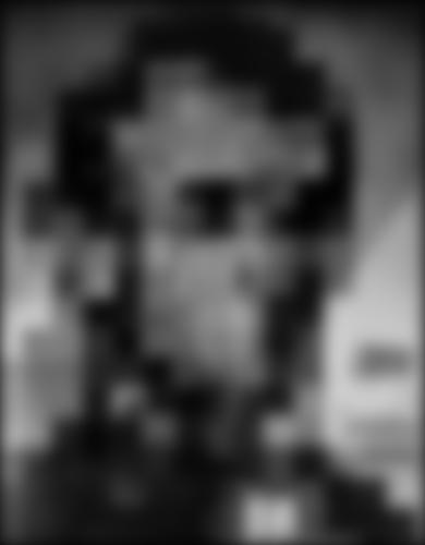
Tiger-RDJ Hybrid

|
|
Gaussian 1

|
Laplacian 1

|
Gaussian 2

|
Laplacian 2

|
Gaussian 3

|
Laplacian 3

|
Gaussian 4

|
Laplacian 4

|
Gaussian 5
|
Laplacian 5

|
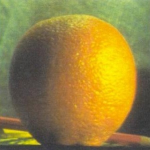
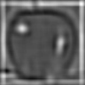
Multiresolution Blending
For this task, I utilized the Gaussian/Laplacian stacks to seamlessly blend two images as described
in the 1983 paper by Burt and Adelson. An image spline, a smooth seam that joins images together
through mild distortion, can be generated by taking advantage of the Gaussian filter. To do this, I
first generated Gaussian and Laplacian stacks for the two input images as well as the mask image, an
image used to determine which parts of the images will be used for multiresolution blending. Then, I
computed the Laplacian stack of the resulting image using the equation
LS_i = GR_i * LA_i + (1 - GR_i) * LB_i, where GR is the Gaussian filtered
mask image and LS, LA, LB are Laplacian images for the result and the input images,
respectively.
Using the equation on five levels, I performed blending separately at each level. Then, taking
advantage of the observation found from the previous task, I summed up the images to generate the
blended image. For this task, I set ksize = 45 and sig = 2, 4, 8, 16, 32,
the same setting as before.
I defined my own imadjust function to make low-contrast images more visible. Below are
the results:
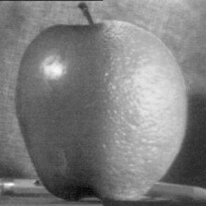
Apple

|
Orange
|
Mask

|
Laplacian(A) 1

|
Laplacian(B) 1

|
Gaussian 1

|
Laplacian(A) 2

|
Laplacian(B) 2

|
Gaussian 2

|
Laplacian(A) 3

|
Laplacian(B) 3

|
Gaussian 3

|
Laplacian(A) 4

|
Laplacian(B) 4

|
Gaussian 4

|
Laplacian(A) 5
|
Laplacian(B) 5

|
Gaussian 5

|
Oraple
|
||
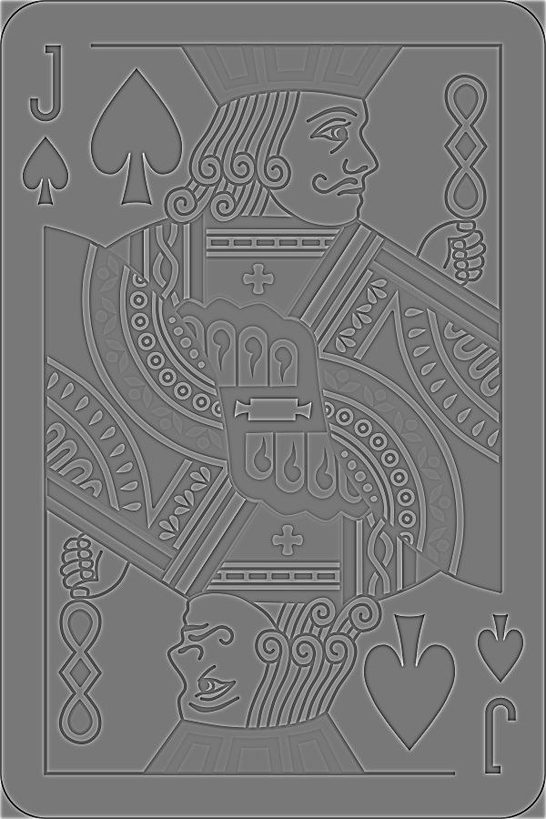
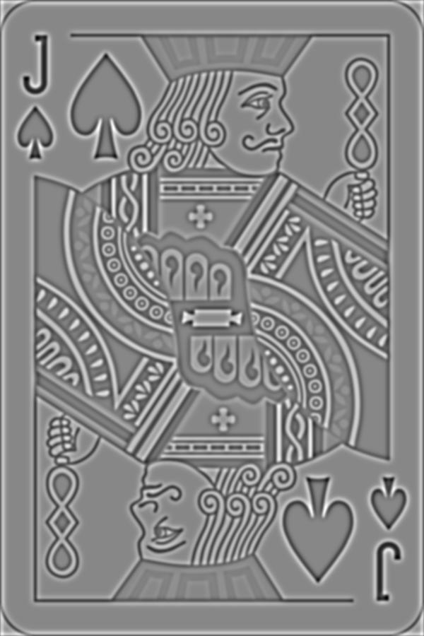
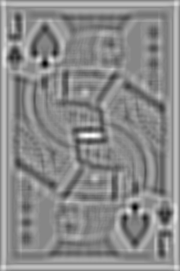
Spades

|
Diamonds

|
Mask

|
Laplacian(A) 1

|
Laplacian(B) 1
|
Gaussian 1

|
Laplacian(A) 2
|
Laplacian(B) 2

|
Gaussian 2

|
Laplacian(A) 3

|
Laplacian(B) 3

|
Gaussian 3

|
Laplacian(A) 4
|
Laplacian(B) 4

|
Gaussian 4

|
Laplacian(A) 5

|
Laplacian(B) 5
|
Gaussian 5

|
Queen of Spadiamonds

|
||
|
Sam
|
Japan
|
Mask

|
Laplacian(A) 1

|
Laplacian(B) 1
|
Gaussian 1

|
Laplacian(A) 2

|
Laplacian(B) 2
|
Gaussian 2

|
Laplacian(A) 3

|
Laplacian(B) 3

|
Gaussian 3

|
Laplacian(A) 4

|
Laplacian(B) 4
|
Gaussian 4

|
Laplacian(A) 5

|
Laplacian(B) 5

|
Gaussian 5

|
Sam at Japan!

|