CS194-26 Project 2: Fun with Filters and Frequencies!

Sairanjith Thalanki | 3032739634 | sthalanki@berkeley.edu | cs194-26-adm

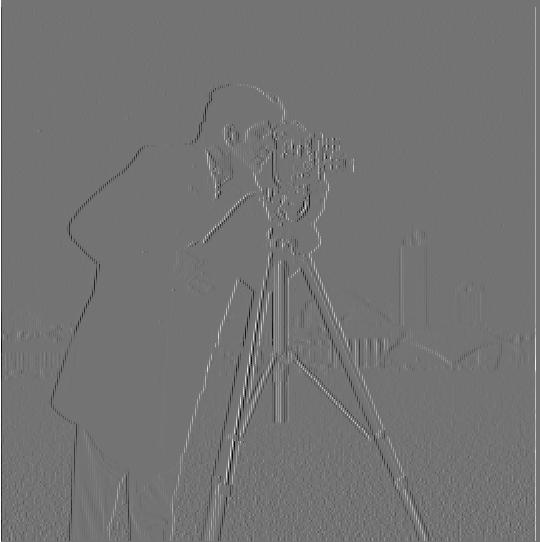
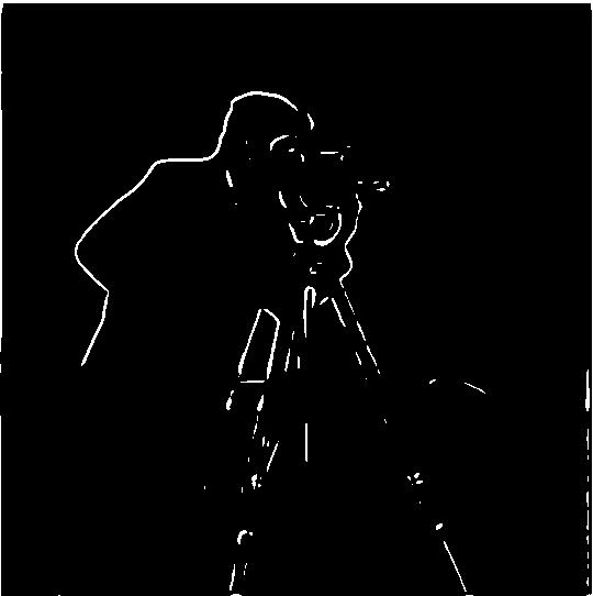
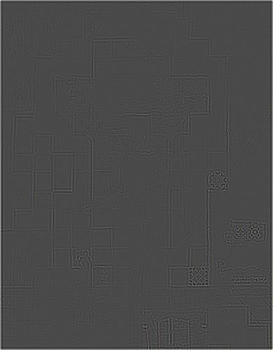
Part 1.1: Finite Difference Operator

I found the partial derivative in x and y of the cameraman image by convolving the image with finite difference operators [1, -1] and [[1], [-1]] which gives us the vertical and horizontal edges respectively. We can then take the partial derivative images and find the gradient magnitude by doing (dx ^2 + dy ^ 2)^(1/2). Finally, to binarize the gradient magnitude image, I replaced all pixels in the gradient magnitude image above a threshold (0.25) to 1 and all other pixels to 0.

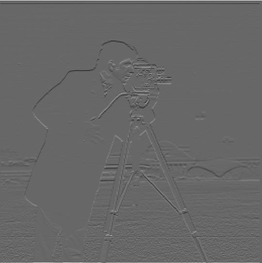
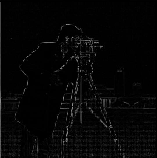
Part 1.2: Derivative of Gaussian (DoG) Filter

You get the same result if you convolve the image with the gaussian filter and then convolve that result with the finite difference operator and if you convolve the gaussian filter and the finite difference operator first and then convolve the image with the combined filter. I used a gaussian kernel with sigma 2 and multiplied the kernel by its transpose to get a 2D gaussian filter to use for blurring. Between part 1.1 and part 1.2, the major difference is there is less noise especially in the grass at the bottom of the image.

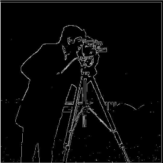
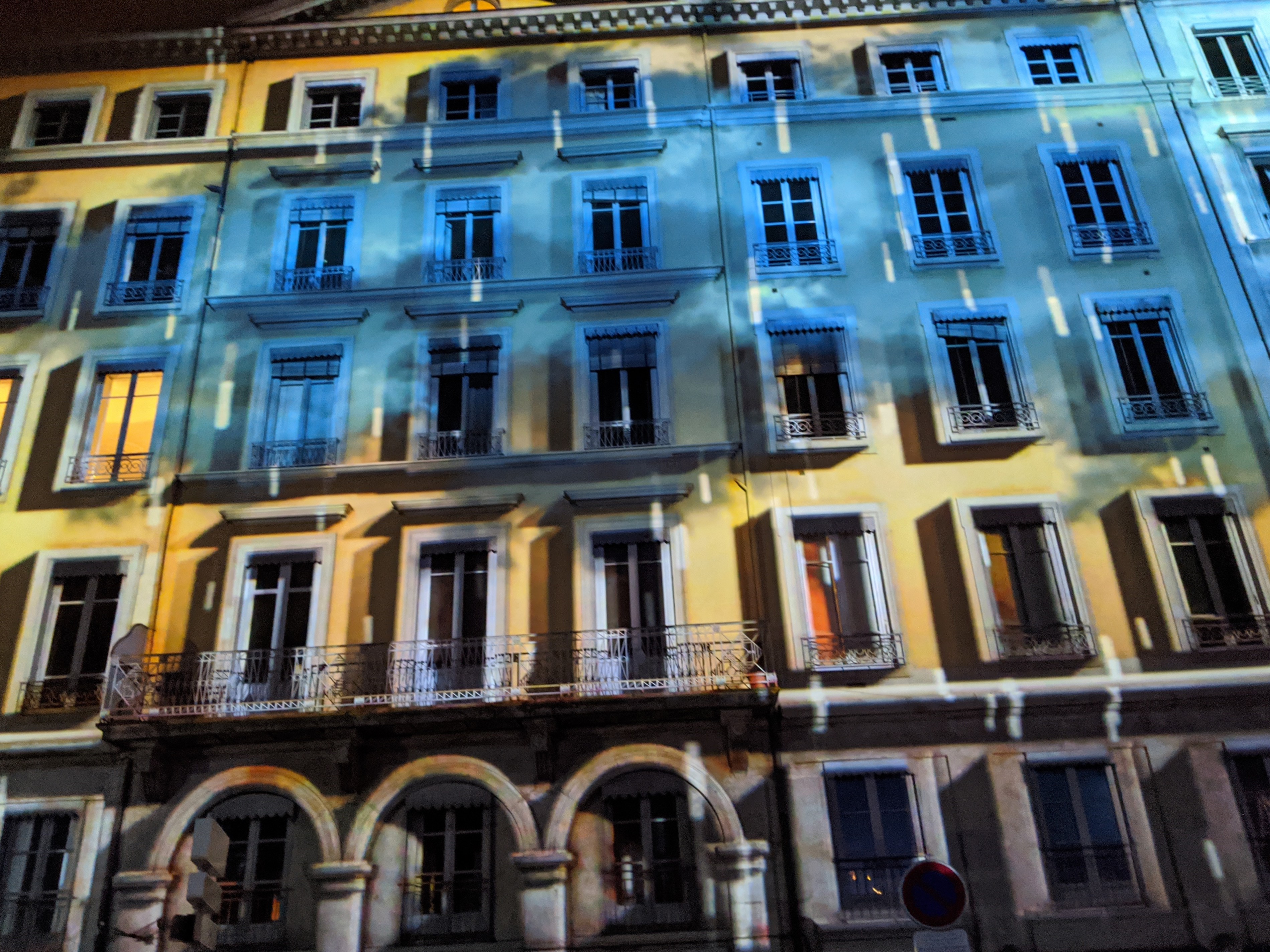
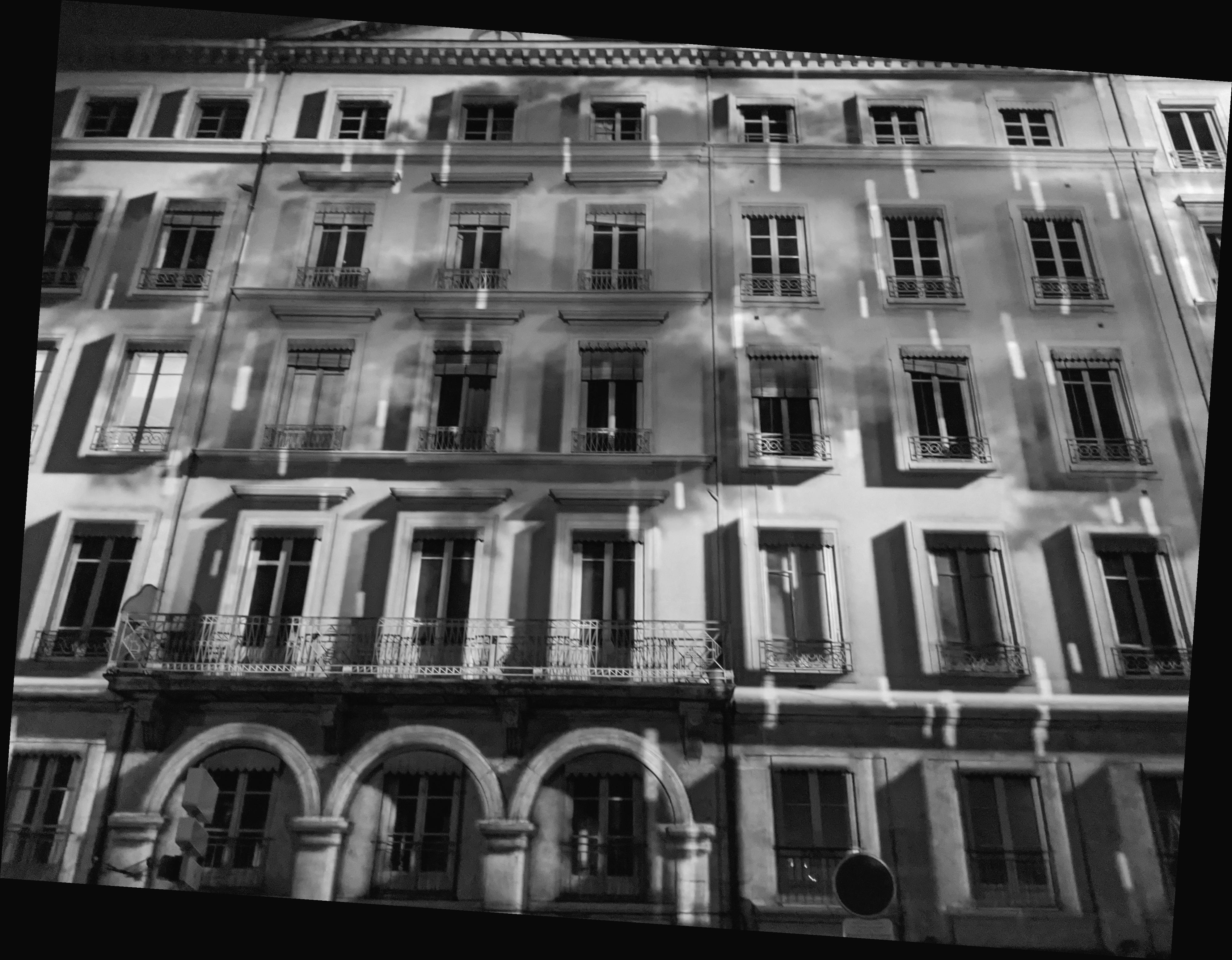
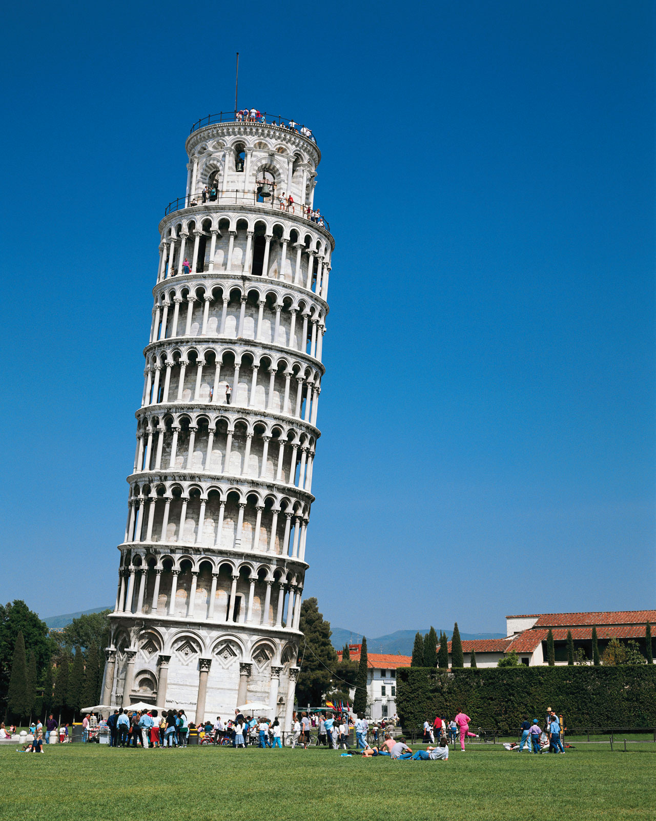
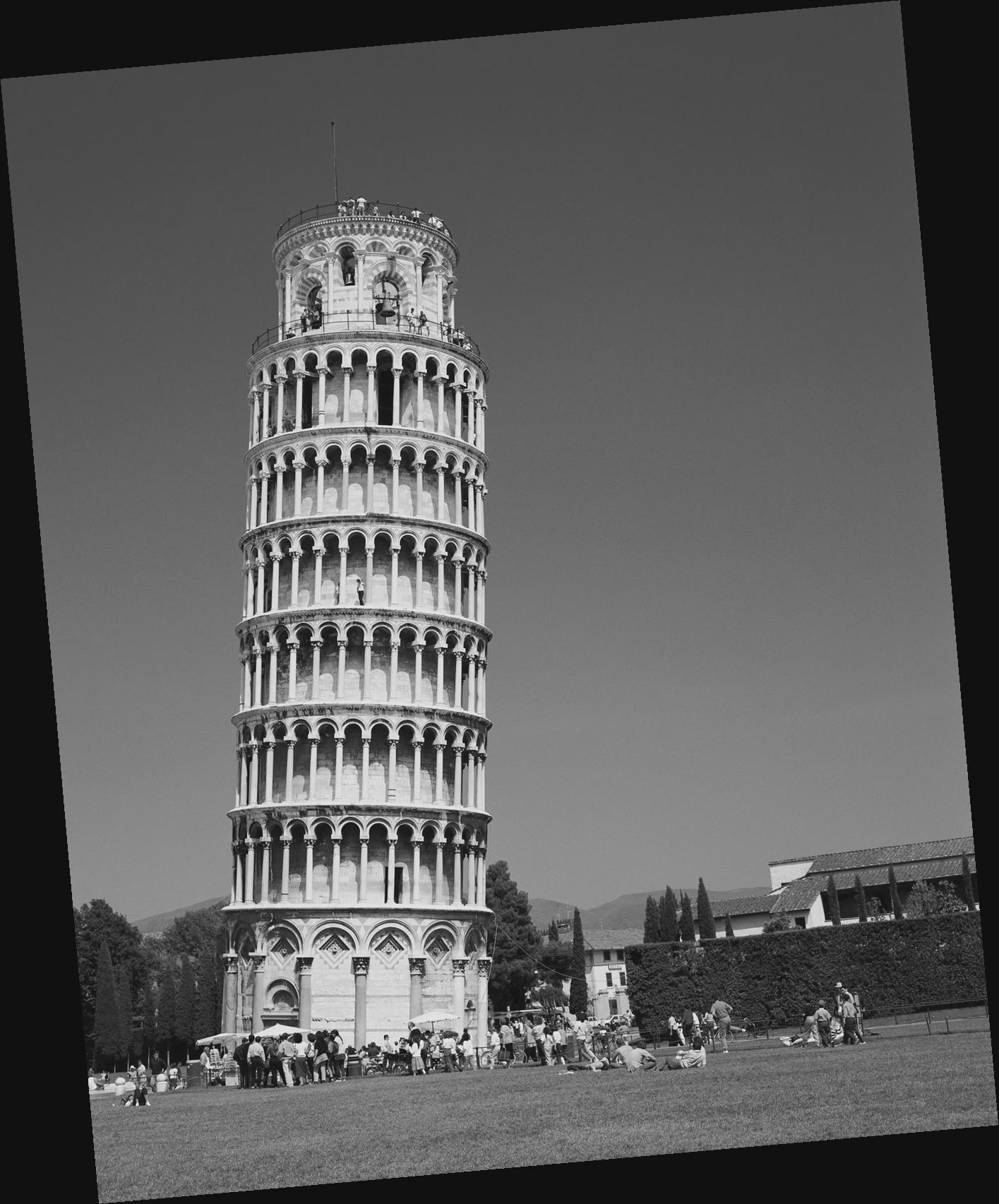
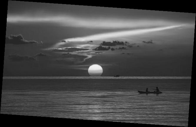
Part 1.3: Image Straightening

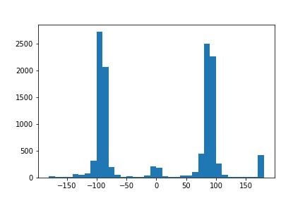
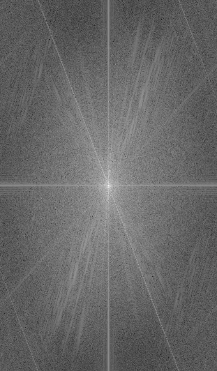
In order to straighten our image, we check which rotation has the greatest number of vertical and horizontal edges (edges with angles close to 0, 90, 180, 270 degrees) because gravity causes many objects to have vertical & horizontal structures to stay balanced. I found that a rotation of -4 degrees led to straightened image.

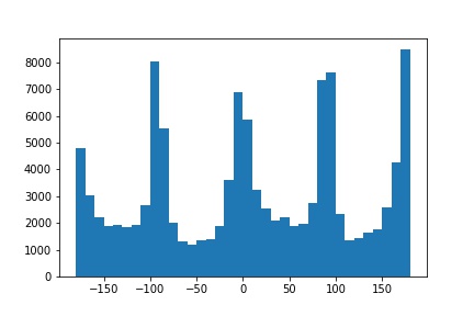
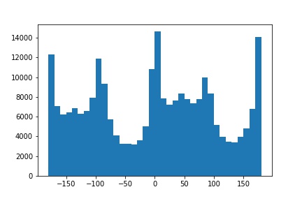
1. First, we loop through all of rotations that we would like to consider. In my case, I looped through either -180 degrees to 180 degrees to check all possible rotations or -45 to 45 if I'm confident that the image is upright and I would like run the code quickly.
2. Next, we compute the gradient angles at every pixel (excluding the black border and any other non-edges by checking if the gradient magnitude is greater than 0.1) by taking arctan2(dy, dx)
3. Finally, we count the number of gradient edges with angles that are within some threshold (5 degrees) of 0, 90, 180, 270 and we pick the rotation with the max count of edges.

The leaning tower of pisa is a failure of the image straightening algorithm since the tower is actually expected to not have vertical and horizontal edges. Thus, when our algorithm straightens the tower (to some extent), it creates something that is not representative of reality.

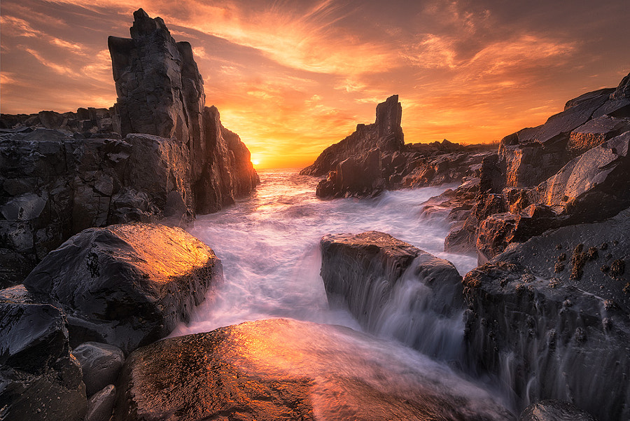
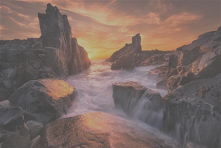
Part 2.1: Image Sharpening

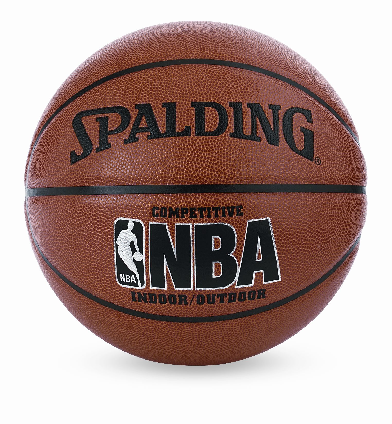
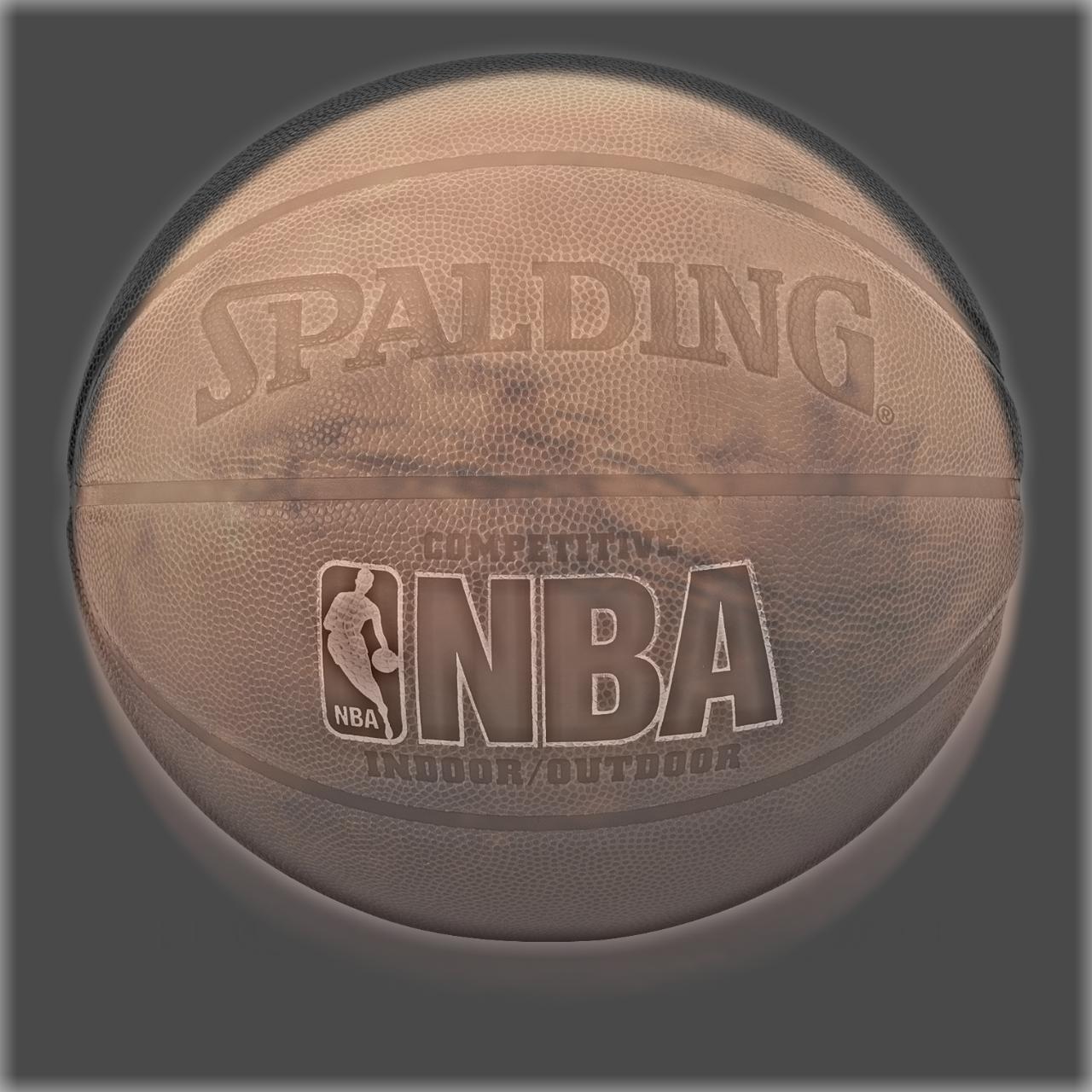
In order to sharpen images, we use the unsharp mask filter. We create this filter by taking (1 + alpha) * unit_impulse - alpha * gauss2D. I used an alpha of 0.75. My observation is that the sharpening makes the image duller but we can also see greater contrast and enhanced edges.

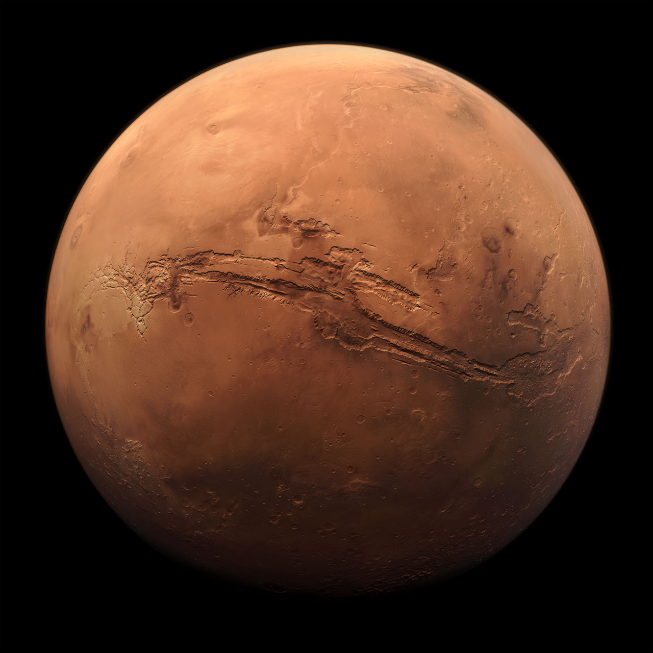
We can see with the rocky landscape below that image sharpening method doesn't recover the original image. There are some artifacts of the sharpening including that the image looks signficantly dimmer and the resolution seems to be lower.

TODO blur sharp image and then resharpen

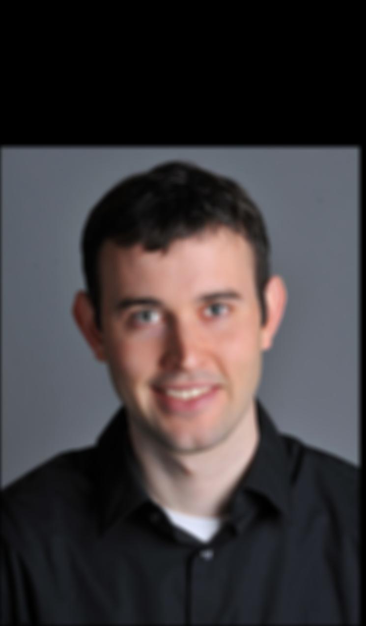
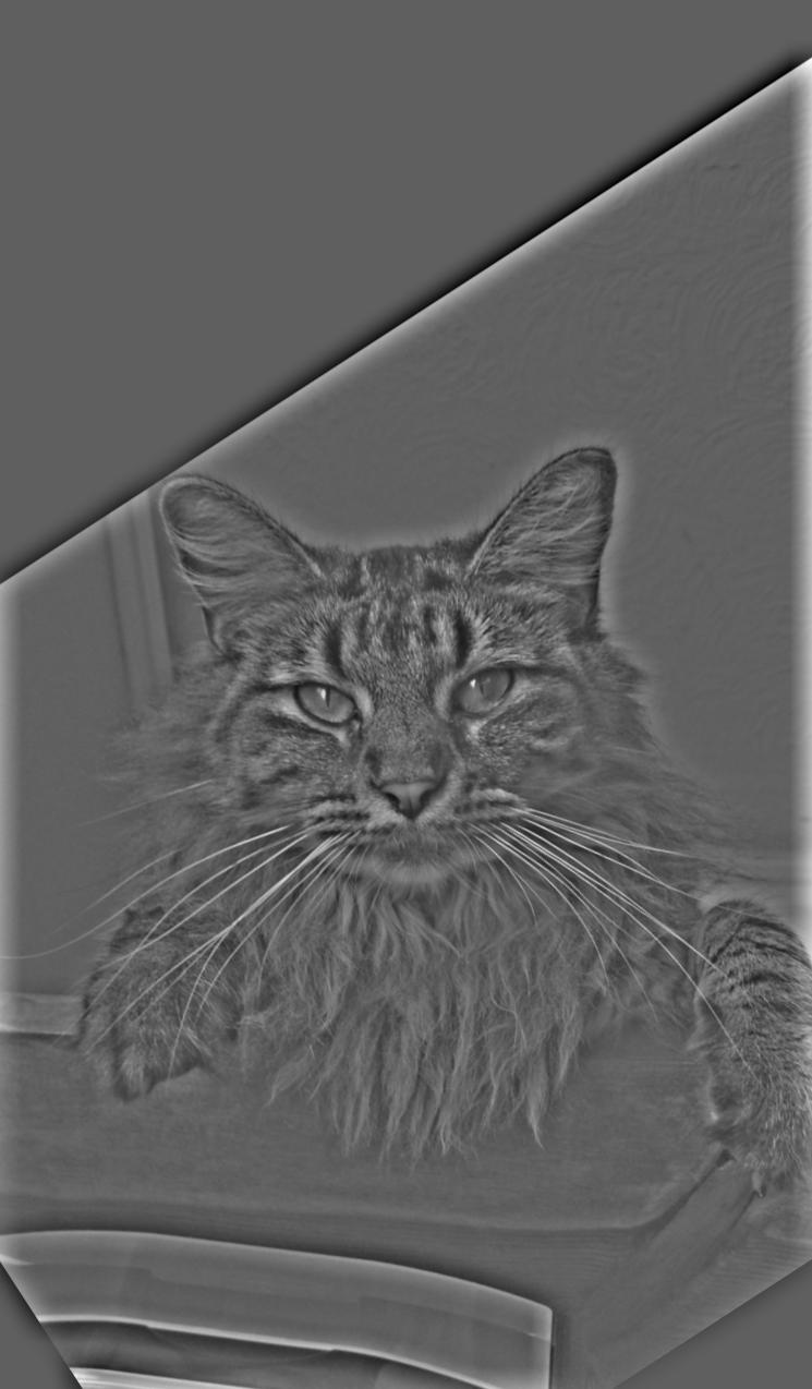
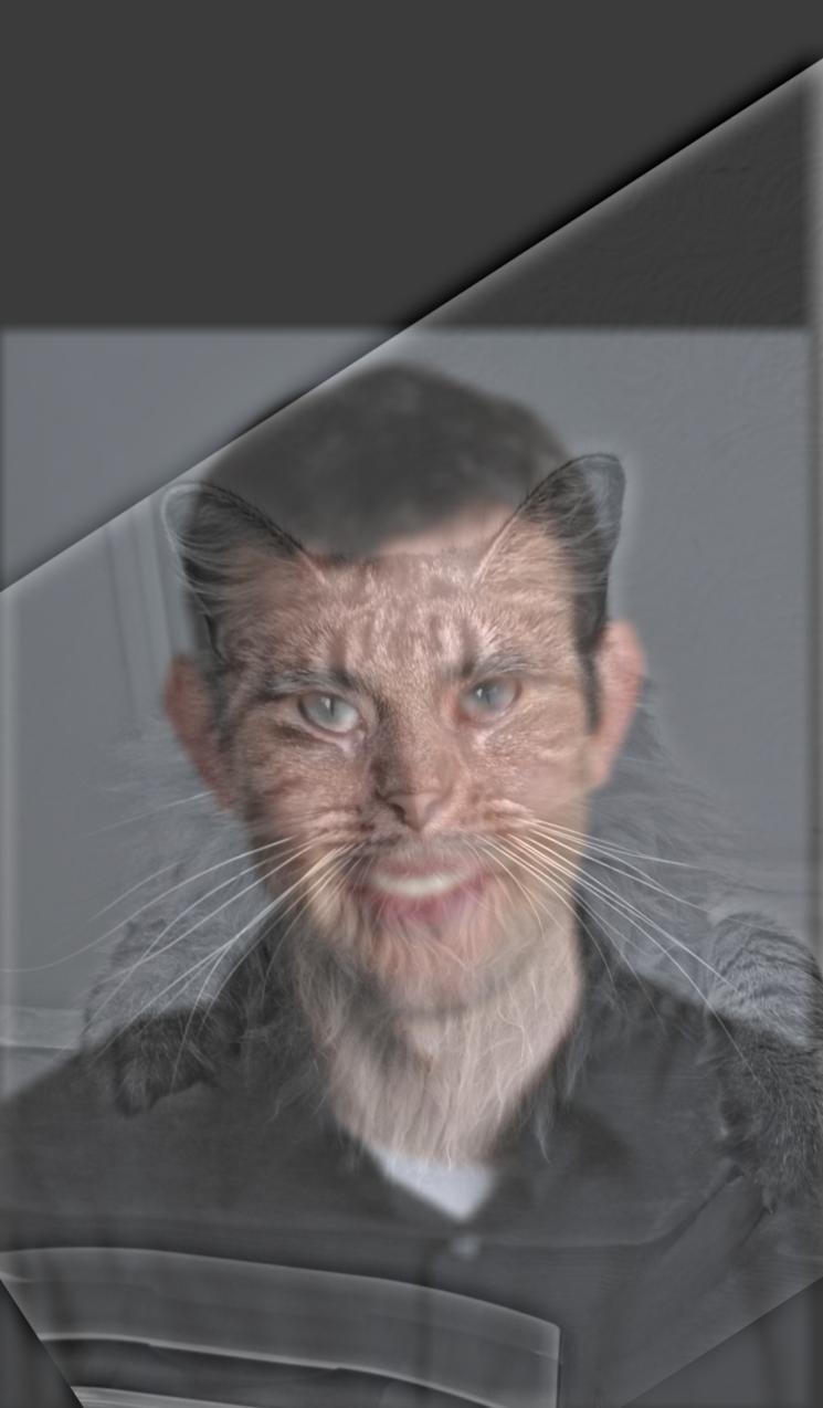
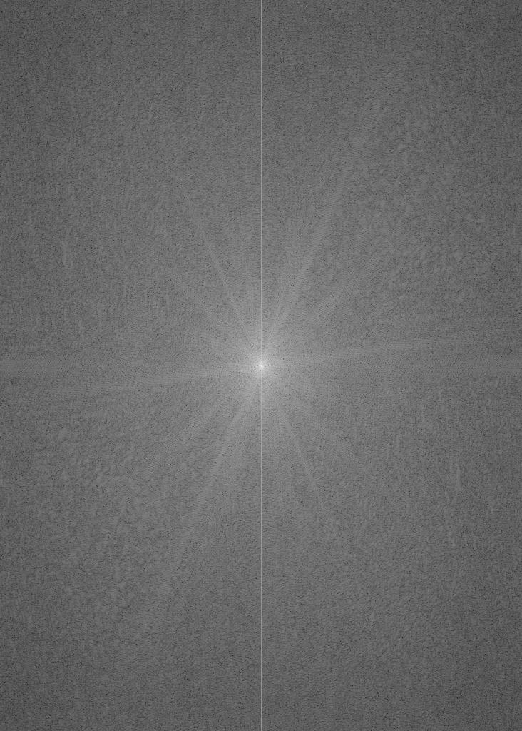
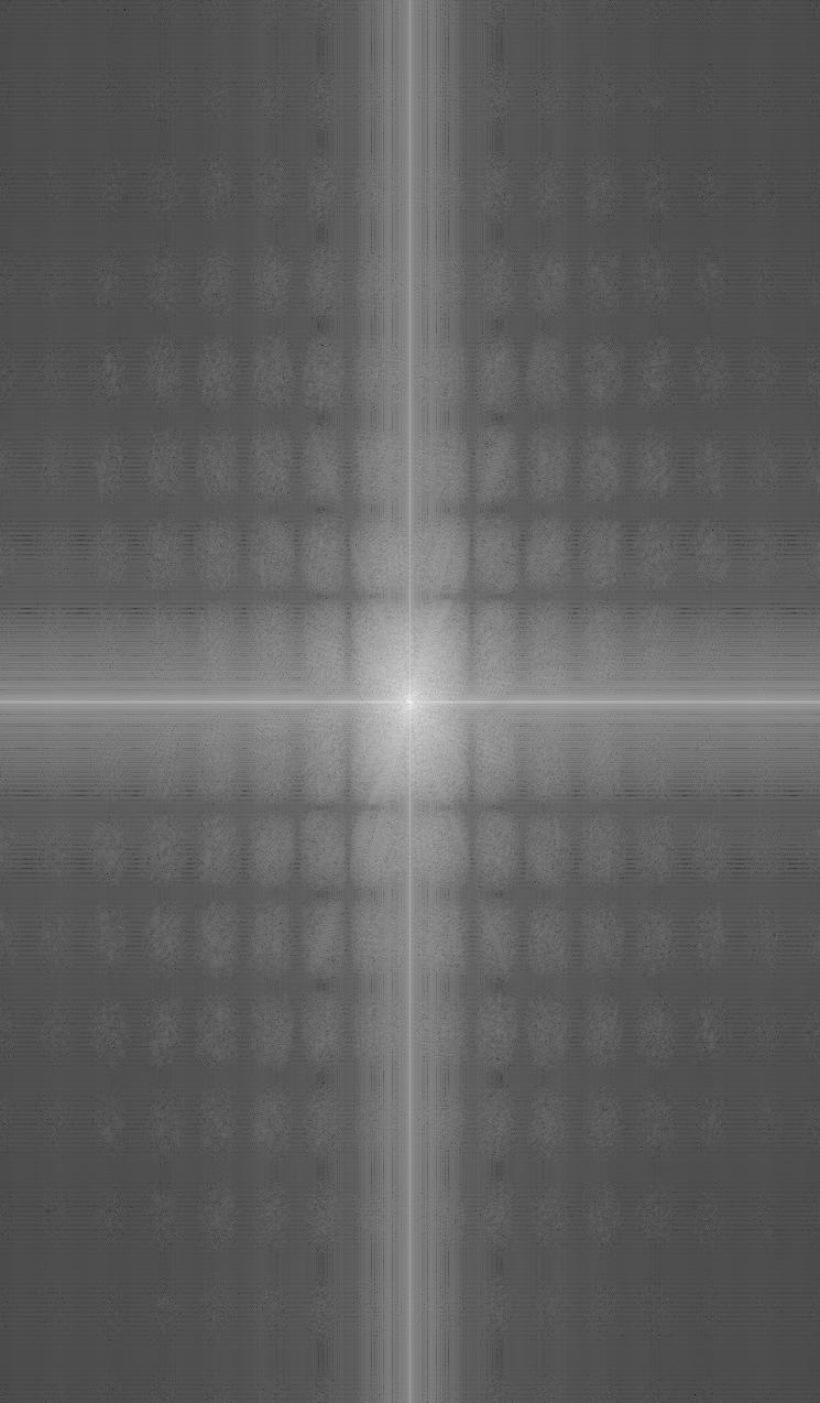
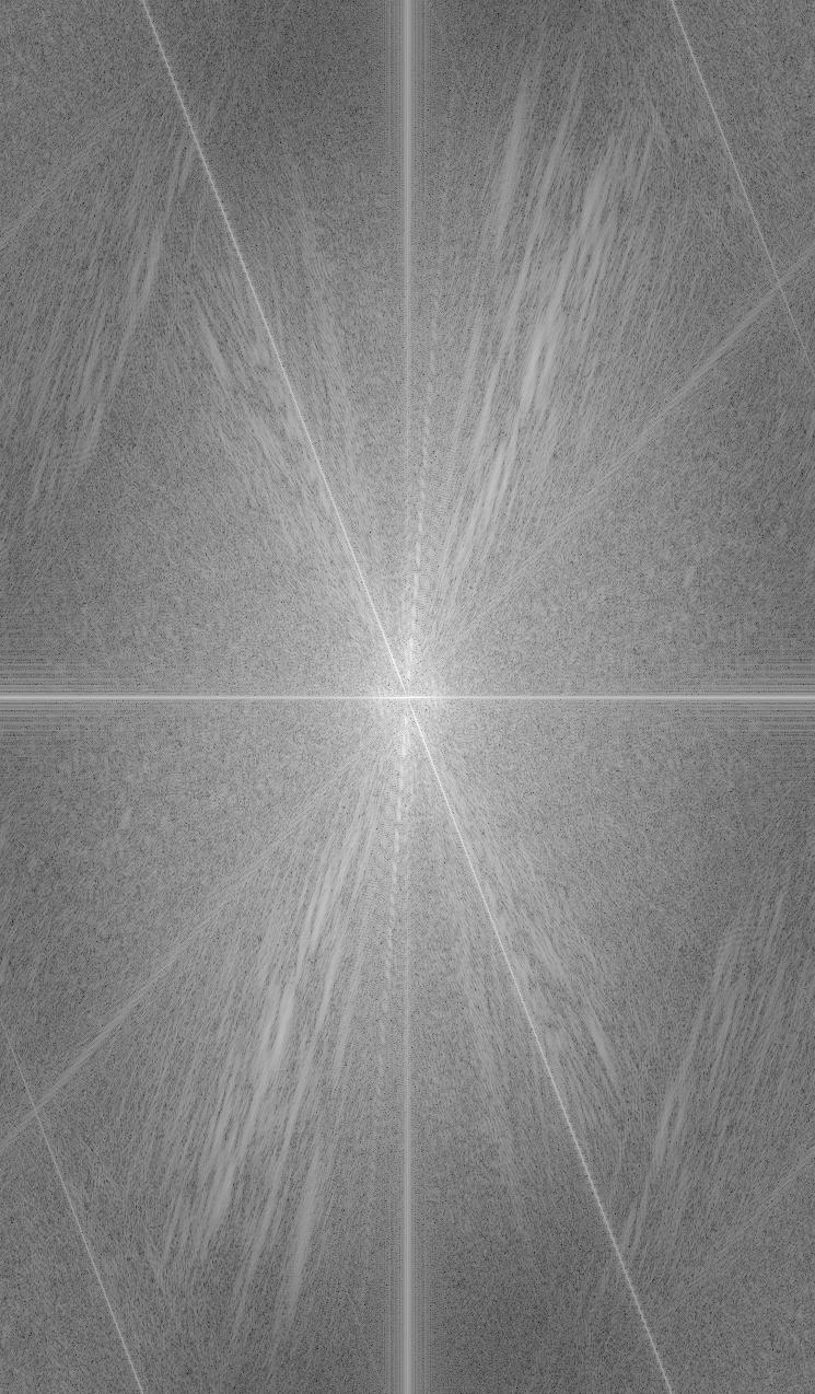
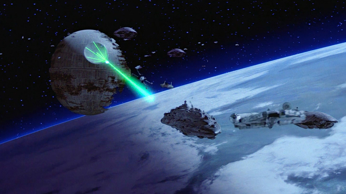
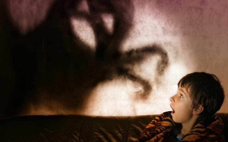
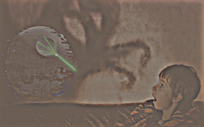
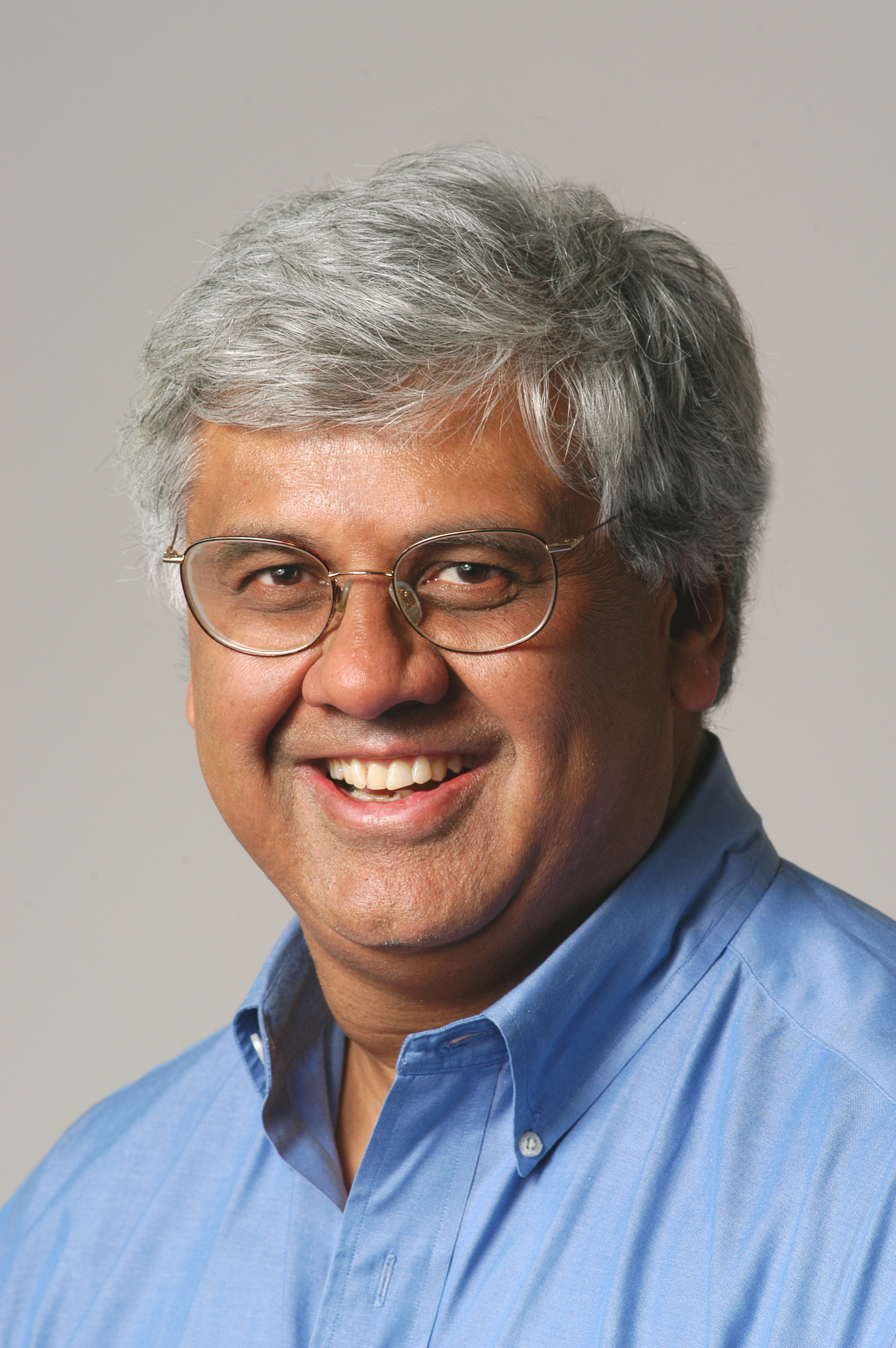
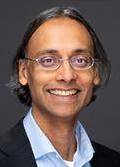
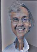
Part 2.2: Hybrid Images

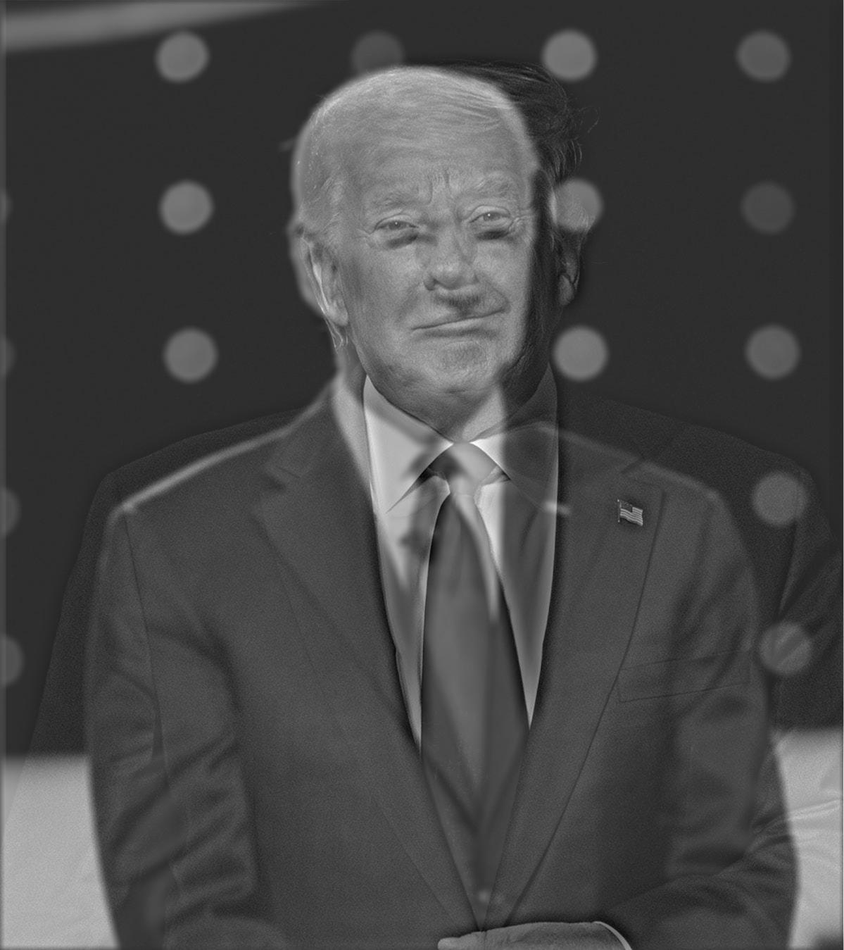
For this section, we are create hybrid images which are 2 images that are "blurred" together so that you see one image at a far away distance (when you see mostly low frequencies) and another image when you are at a close distance (when you see mostly high frequencies). We acheive this by applying a gaussian blur on the first image and the convolving a laplacian (unit impulse - gaussian blur) with the second image. We add the 2 images together to get the hybrid iamge. I used sigma1 = 7 and sigma2 = 20 to generate the gaussian kernels I used for the low pass and high pass filter. The hybrid of Donald Trump and Joe Biden did not look as good as the other hybrid images since the two images didn't align.

Frequencies

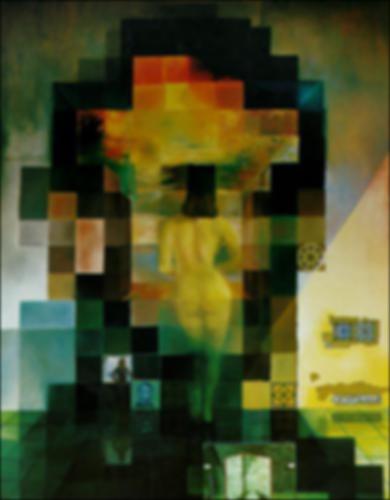
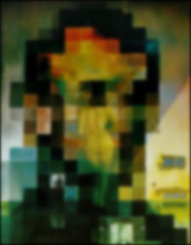
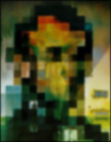
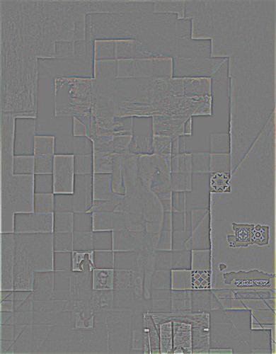
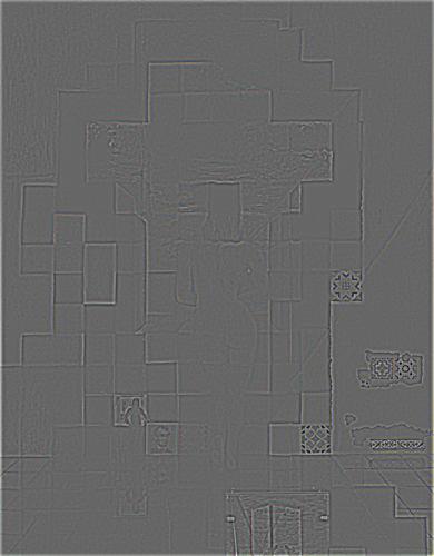
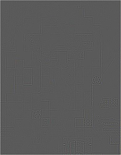
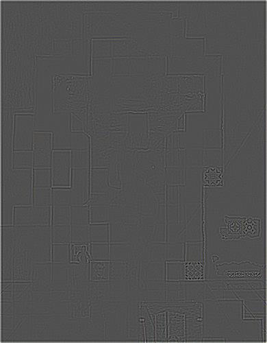
Part 2.3: Gaussian and Laplacian Stacks

In this part, I created a Gaussian and a Laplacian stack using sigma 2 for both. I created the gaussian stack by convolving the gaussian kernel with itself n times for n levels. I then applied the new filter on the image. Next, I created the laplacian stack by creating a new filter which is the unit impulse minus the gaussian kernel. I convolved this filter with itself n times and then applied it on the image.

Part 2.4: Multiresolution Blending

For the multiresolution blending, we use the gaussian & laplacian stacks we implemented in the last section and this equation LS_l = GR * LA + (1 - GR) * LB at every level and sum up all of the levels to get an image spline. GR is the convolution between the mask and the gaussian stack and LA/LB is the laplacian stack convolved with the respective image.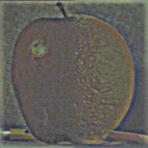

The most important thing I learned in this project is how to use gaussian and laplacians to blur/sharpen images and how to use those filters to combine images in a sensible way.