
Overview
In this project we undertake a journey to explore (and play) with image frequencies. We will implement the Gaussian filter and use it as our foundation for more advanced applications such as edge detection, sharpening, and image blending. Real applications of these concepts can be found in photo processing applications such as Photoshop, and in built-in features of some prosumer cameras and smartphones.
PART 1: Fun with Filters
Part 1.1: Finite Difference Operator
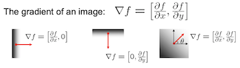
We are interested in detecting the edges of an image. In principle, edge detection relies of detecting sudden changes of contrast or brightness from one area of the image to another. To achieve this, we use the finite difference operator to generate two derivative images with respect to the x and y axis.
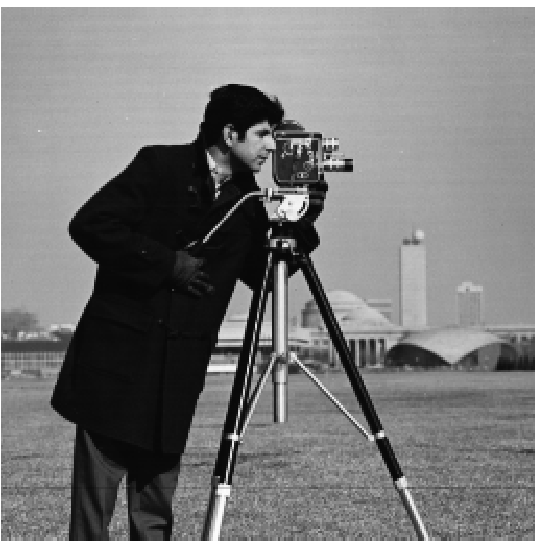 Target image. |
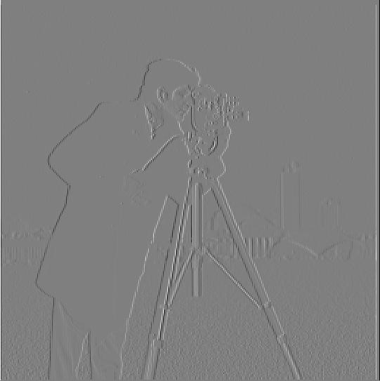
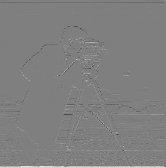
First, we convolve the original image with the finite difference operator in the x dimension: [1, -1], then we convolve the image with the finite difference operator in the y dimension: [[1], [-1]].
 Differential and vector forms. |
 This reveals edges along the x-axis. |
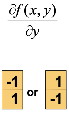 Differential and vector forms. |
 This reveals edges along the y-axis. |
Then, we compute the gradient magnitude by using a simple adaptation of the Pythagorean Theorem where we input our two partial derivatives from the previous step.
 Visual representation. |
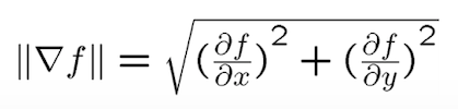 Pythagorean Theorem. |
Finally, we binarize the gradient magnitude image by picking an appropriate threshold. This reduce noise and isolate the edges. The final edge image is shown below at the right hand side.
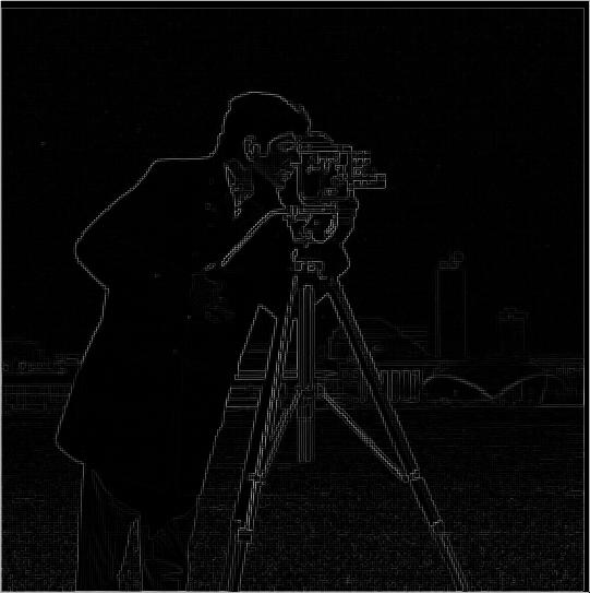 The edges are dim but visible. |
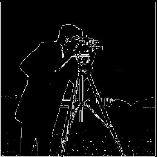 The edges are visible. |
Part 1.2: Derivative of Gaussian (DoG) Filter
Although our previous technique for detecting edges worked at some extent, we realize that the final edge image still has some noise manifested as tiny white dots and lines. We know that edges located in areas where there are a sharp, sudden changes in contrast (high frequencies), but sometimes images can be “busy,” which mean that some image areas with lots of subtle detail can fool out naive algorithm to think they are actually edges. This grainy fuzziness can be attenuated easily by smoothing the image. One technique to smooth images is by applying a gaussian blur, which acts as a low-pass filter on the image while preserving boundaries and edges better. To generate a gaussian filter we use the formula shown below, where x is the distance from the origin in the horizontal axis, y is the distance from the origin in the vertical axis, and σ (sigma) is the standard deviation of the Gaussian distribution. When applied in two dimensions, this formula produces a surface whose contours are concentric circles with a Gaussian distribution from the center point as shown in the following diagram:
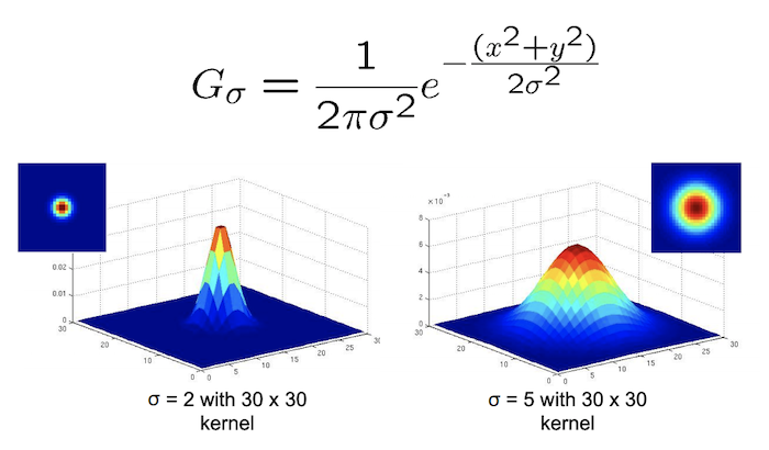 In two dimensions, the formula of a gaussian is the product of two one-dimensional Gaussian functions. |
The values from this distribution are used to build a convolution matrix which is applied to the target image. This will generate a blurred image where each pixel's value is set to a weighted average of that pixel's neighborhood. Then, we convolve the blurred image with the finite difference operators just as in Part 1.1 to get the two partial derivatives, which then are used to get the gradient magnitude. The results of this multi-convolution process are shown in the images below:
|
Target image. |
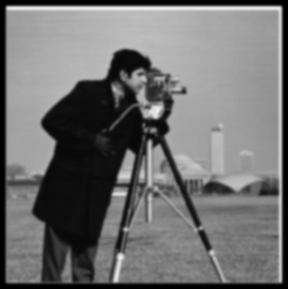 Gaussian filter was applied. |
 Edges are now much clearer, with less noise. |
What differences do we see compared to the previous part? As we can see, the edges are now much more pronounced and there is visibly less noise in the image than our naive approach in part 1.1. We can achieve this result with a single convolution instead of two by creating a Derivative of Gaussian (DoG) filter. To do this, we convolve the gaussian kernel we generated above with the finite difference operators D_x and D_y to get our DoG filter.
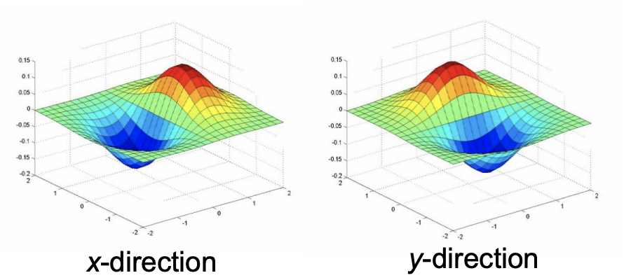 Finite difference operators D_x and D_y. |
 Finite difference operator for x-axis. |
 Finite difference operator for y-axis. |
Finally, we convolve our original image with our newly created Derivative of Gaussian (DoG) filter, and we see that the result is exactly the same as when we first applied the gaussian filter to the original image, while avoiding an additional convolution computation! Note that convoluting our finite difference operators is computationally cheaper than applying a gaussian blur to the target image first.
|
Target image. |
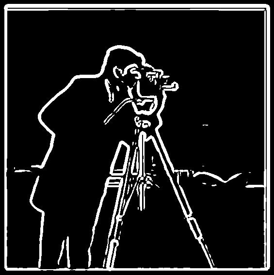 Edges are now much clearer, with less noise. |
Part 1.3: Image Straightening
In part 1.2 we explored how the gradient magnitude can be used to detect edges. In this section now we will explore how gradient direction can be used for image straightening. Instead of computing the magnitude of the two axial gradient components, we will them to compute the angle to figure out the direction of contrast change at a given location of an image. To compute the angles, we use the following formula:
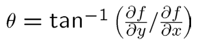 The gradient angle is defined as the direction of maximum change. |
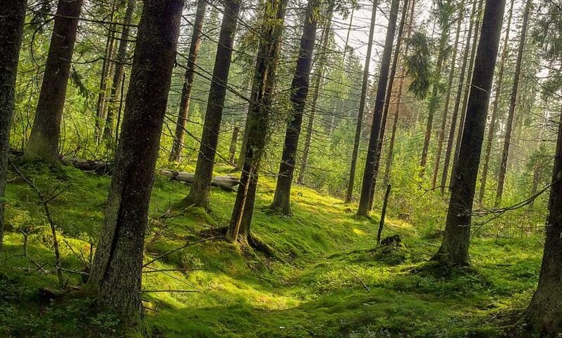
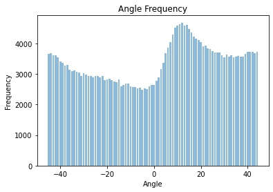
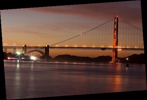
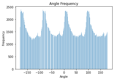
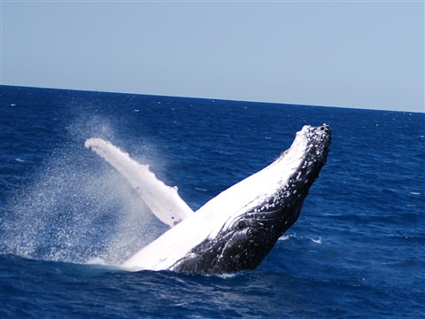
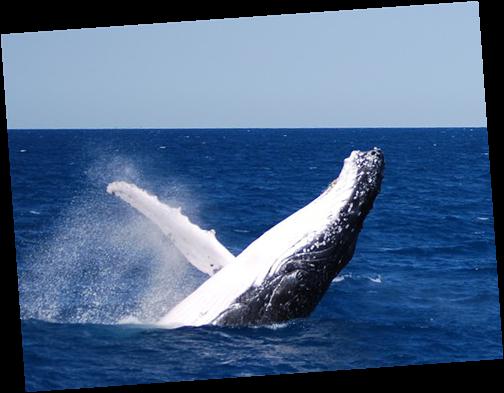
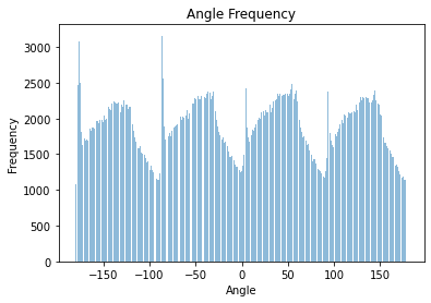
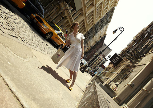
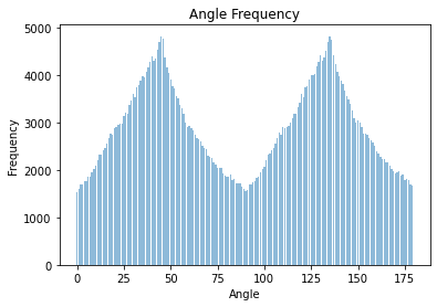
As most pictures have an horizon line (ground, waterline, etc.) and structures parallel to it like buildings, trees, people, etc. we can assume that an straightened image will have most edge directions at 0°, ± 90°, ± 180° with respect to the standard cartesian plane (where the x-axis is the floor level). To automatically straighten an image, we rotate the image and compute all the gradient directions at each angle. We then choose the angle that produces the most vertical and horizontal lines. In the example below we show some examples showing the original image, the straightened version, and a graph showing the number of perpendicular angles per angle.
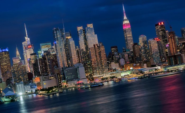 Target Image. |
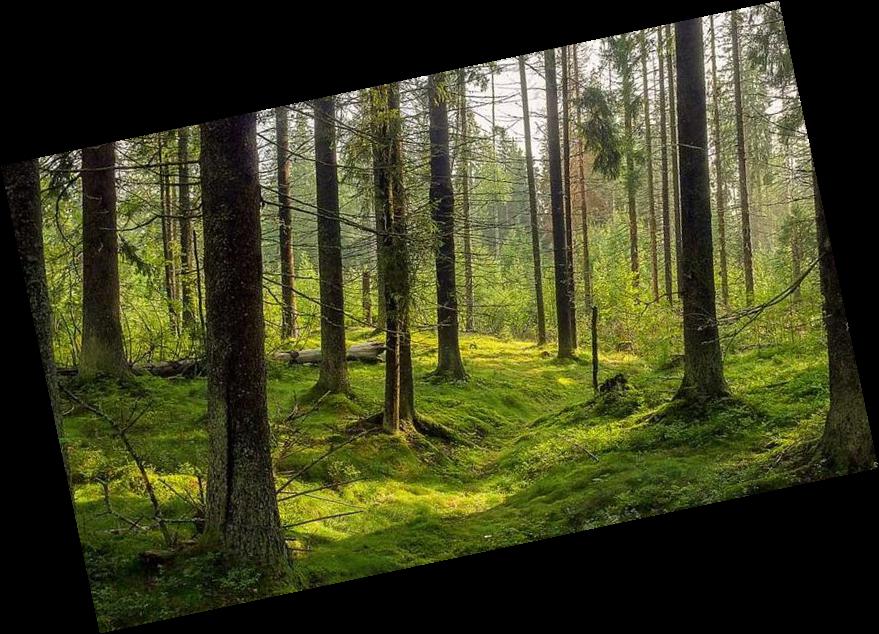
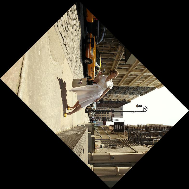
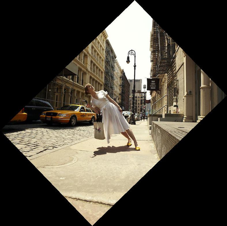
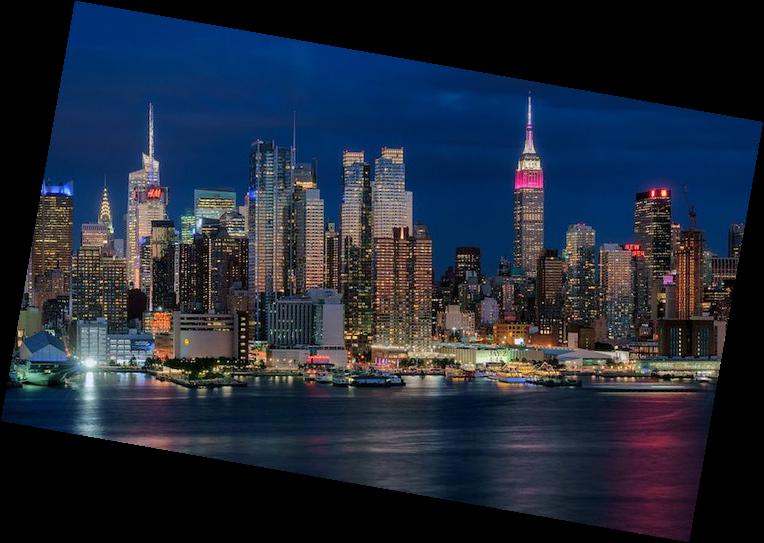 Target Image rotated |
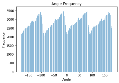 Horizontal and vertical edges are defined to have angles: 0°, ± 90°, ± 180° |
||
 Target Image. |
 Target Image rotated |
 Horizontal and vertical edges are defined to have angles: 0°, ± 90°, ± 180° |
||
 Target Image. |
 Target Image rotated |
 Horizontal and vertical edges are defined to have angles: 0°, ± 90°, ± 180° |
||
 Target Image. |
 Target Image rotated |
 Horizontal and vertical edges are defined to have angles: 0°, ± 90°, ± 180° |
 Target Image. |
 Target Image rotated |
 Horizontal and vertical edges are defined to have angles: 0°, ± 90°, ± 180° |
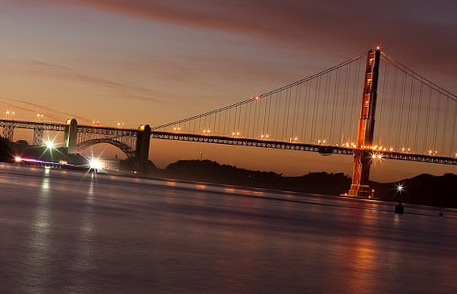
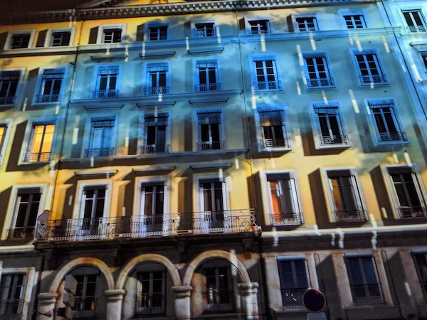
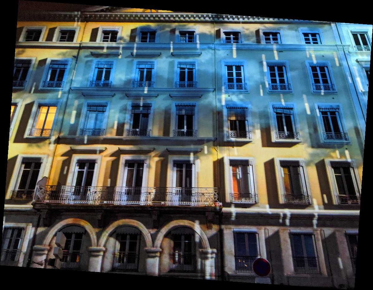
Failure case: Although this algorithm works for may images, there are some images where most lines are in diagonal directions, or the number of vertical and horizontal angles are so close that the algorithm cannot discern if a given right angle correspond to the horizontal or vertical axis. As result, some images can be rotated in the wrong direction. In the following example, the buildings and street floor produce similar number of vertical and horizontal edges in two configurations, the wrong one is shown below.
 Target image. |
 Target Image rotated. |
 Horizontal and vertical edges are defined to have angles: 0°, ± 90°, ± 180° |
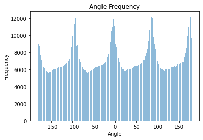
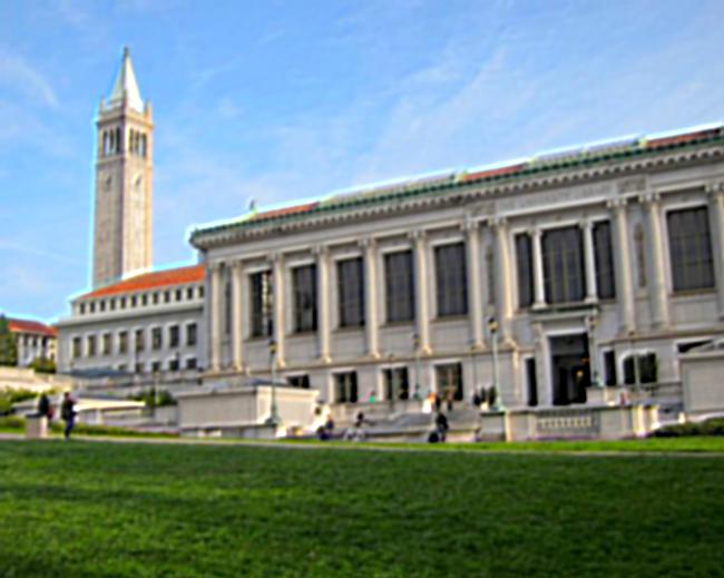
We can fix this by reducing the range of angle rotations or by setting a bias towards a particular direction of rotation. In this case we provide a counterclockwise rotation bias to get the correct angle.
 Target Image rotated. |
PART 2: Fun with Frequencies!
Part 2.1: Image "Sharpening"
In part 1 of this project, we got the chance to get our feet wet on frequencies. Now that we know what a Gaussian filter is, we can further exploit its capabilities to develop additional image manipulation applications. In this section we explore how we can construct a high frequency filter using a gaussian filter, which then will be used to make images sharper. Image sharpening refers to the process of accentuating strong edges (high frequencies) and some small details so that they become more visible to the human eye. The fovea in our eyes is a tiny pit located in the macula of the retina where visual detail is resolved. In other words, it is the area in our eye in change of decoding high frequencies (details).
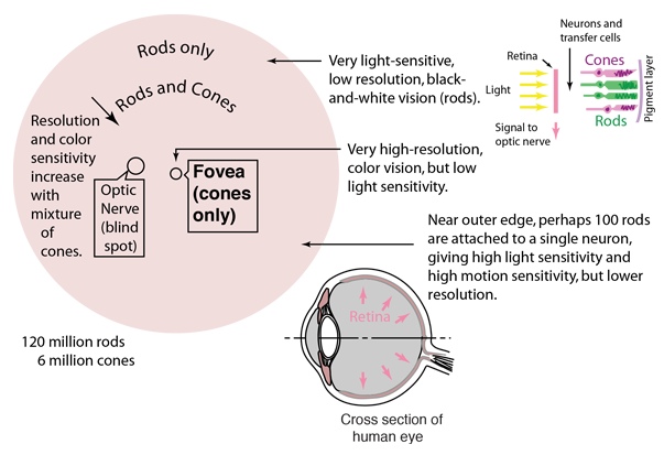 The fovea is the central region of the eye. |
In order to enhance the details of an image, we extract its high frequencies and then we add it back by some constant factor. To get the high frequencies from an image we first get its low frequencies by applying a gaussian blur filter on the original image and then we subtract the resulting blurred image from the original image. We can combine these steps into a single convolution operation called the Unsharp Mask Filter, whose equation is shown below. The gaussian kernel is expressed as g, the original image as f, the multiplicative factor as α (alpha), and the unit impulse matrix as e.
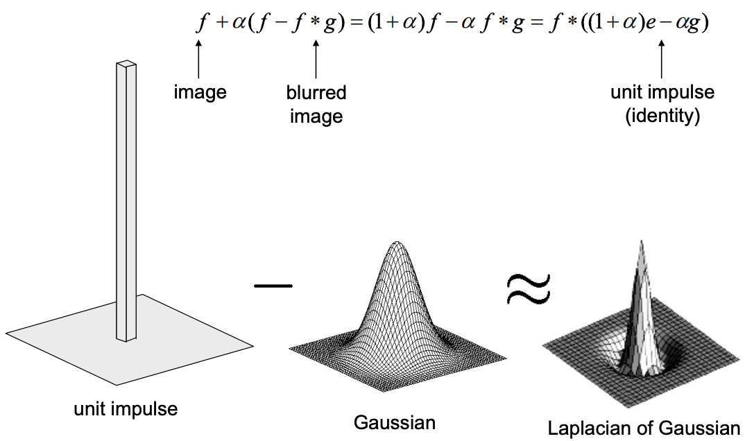 Note: The unit impulse matrix is a matrix where the central cell is 1 and the rest is all zeros. |
By setting the right size and standard deviation for our gaussian kernel, and the right multiplicative factor α (alpha), we can make any image appear sharper. Below we show a Taj Mahal image where the gaussian kernel is of size 35 and σ = 20 at different α values. We also show some additional examples.
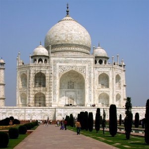 Target image. |
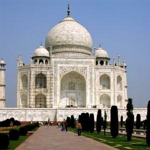 High frequencies are boosted. |
 Image starts to show undesired effects at high contrast areas. |
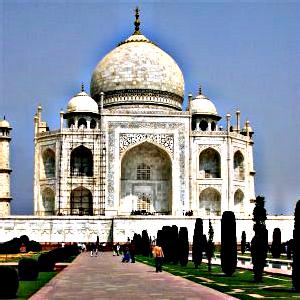 Image is completely overtaken by the high frequencies. |
|||
 Target image. |
 High frequencies are boosted. ksize = 35, σ = 3, α = 0.7 |
 Target image. |
 High frequencies are boosted. ksize = 10, σ = 1.5, α = 2.3 |
It is important to note this process is not a true sharpening technique, as no new information is provided. Unlike image stacking techniques frequently used by astronomers or astrophotographers where new data is provided by additional images to enhance picture quality, our algorithm only enhance the available high frequencies of the images, which may not produce the desired result, and might even increase noise. To show this, we blurred an otherwise sharp image and we use it as input to our algorithm to make it sharper. The result, as you can see below, is not very appealing when compared to the original image.
 Target Image. |
 Gaussian blue applied to target image ksize = 20, σ = 1.9 |
 The result is not very appealing. This is normal due to the lack of new information. ksize = 20, σ = 1.1, α = 6.5 |
Part 2.2: Hybrid Images
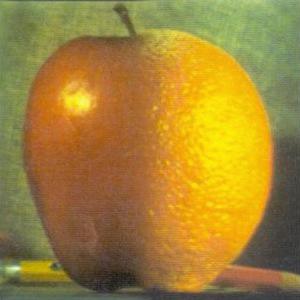
Now that we know how to extract low and high frequencies from images, we can have a little fun! In this section we will create hybrid images, some of which appear to morph when seeing it at different distances. The process to create these images is quite straightforward, with the challenge being finding images that would match well together and finding their right gaussian kernel size and standard deviation σ (sigma). The examples below show how we can make morph between different subjects, and some examples even appear to be different from distance.
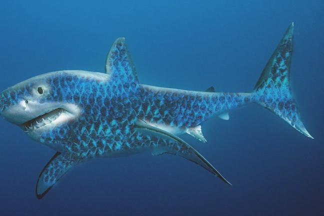
 We extract the low frequency from this image. |
 Hybrid Image ksize = 30, Lσ = 4.55, Hσ = 13.66 |
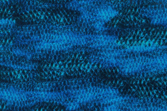
 We extract the high frequency from this image. |
||
 We extract the low frequency from this image. |
 Hybrid Image ksize = 20, Lσ = 12, Hσ = 17 |
We extract the high frequency from this image. |
Bells & whistles:
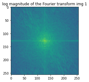
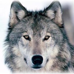
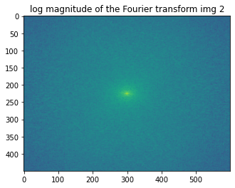
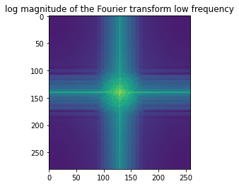
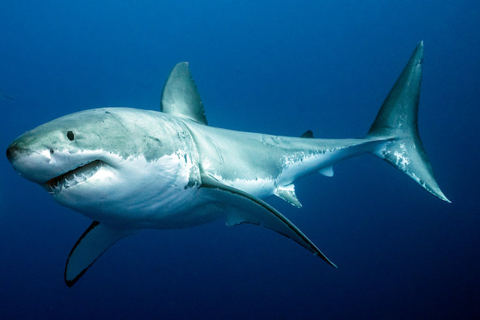
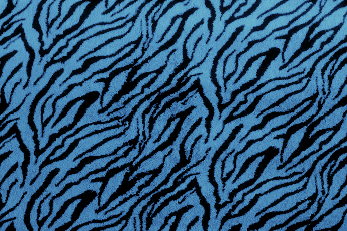
In order to improve the morphing effect, we create colorful hybrid images where we retain the color of the image whose low-frequency component is desired. The high frequency from the second image remains the same regardless of whether the image is colored or in grayscale. For the following image, we illustrate the process through frequency analysis. We show the log magnitude of the Fourier transform of the two input images, the filtered images, and the hybrid image.
|
Target image 1. |
 Log magnitude of the Fourier transform for this image. |
 Target image 2. |
 Log magnitude of the Fourier transform for this image. |
|||
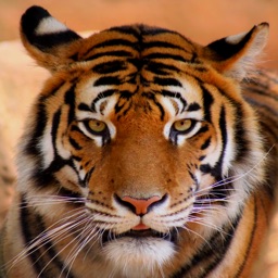
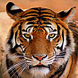
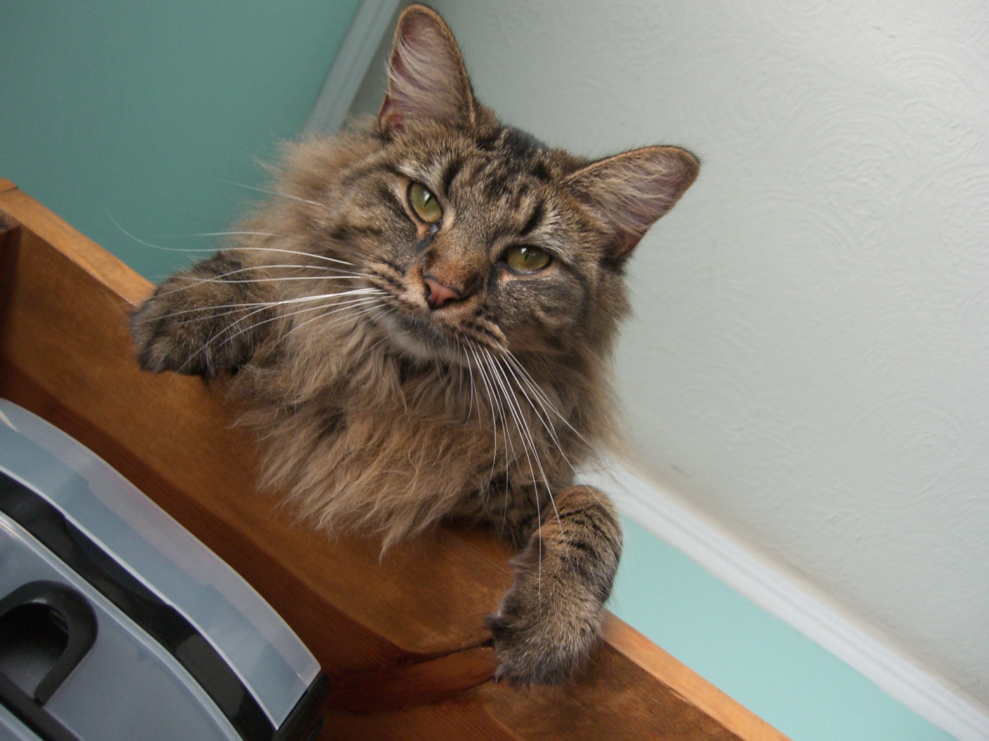
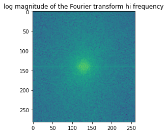
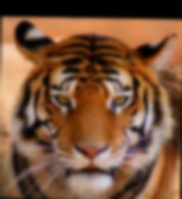 The color for tiger was preserved. ksize = 30, Lσ = 2.55 |
 Log magnitude of the Fourier transform for this image. |
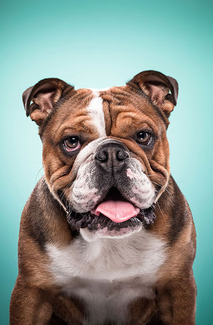
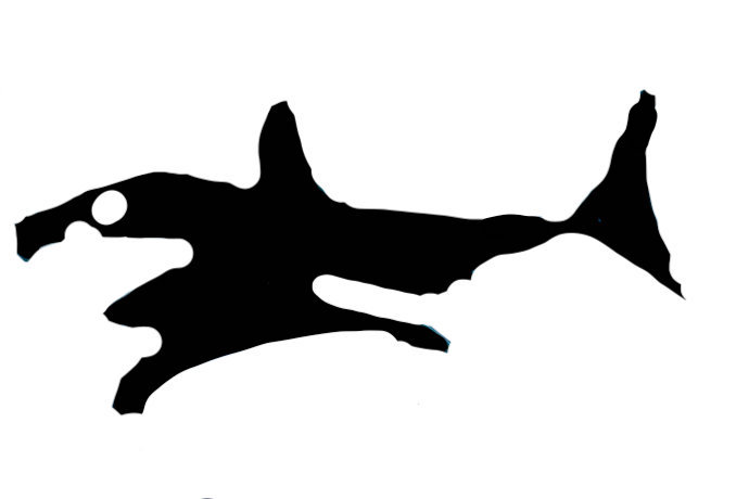
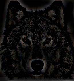 The edges for wolf were preserved. ksize = 30, Hσ = 13.66 |
 Log magnitude of the Fourier transform for this image. |
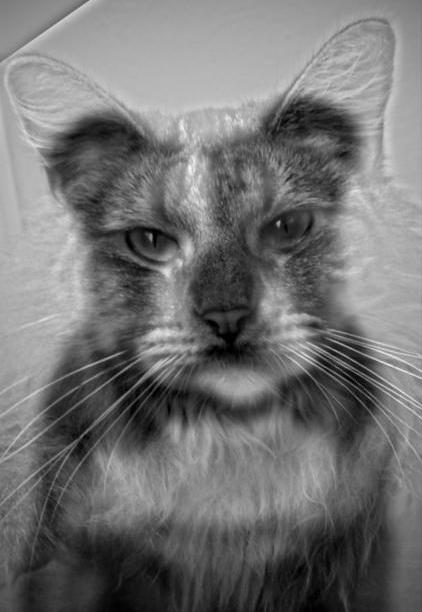
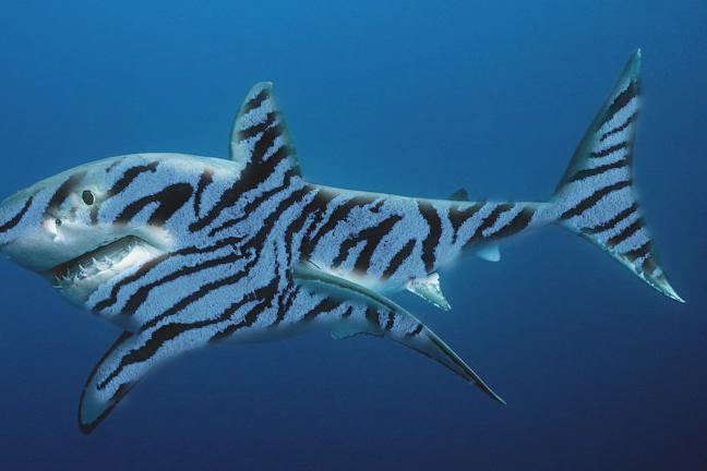
Final result
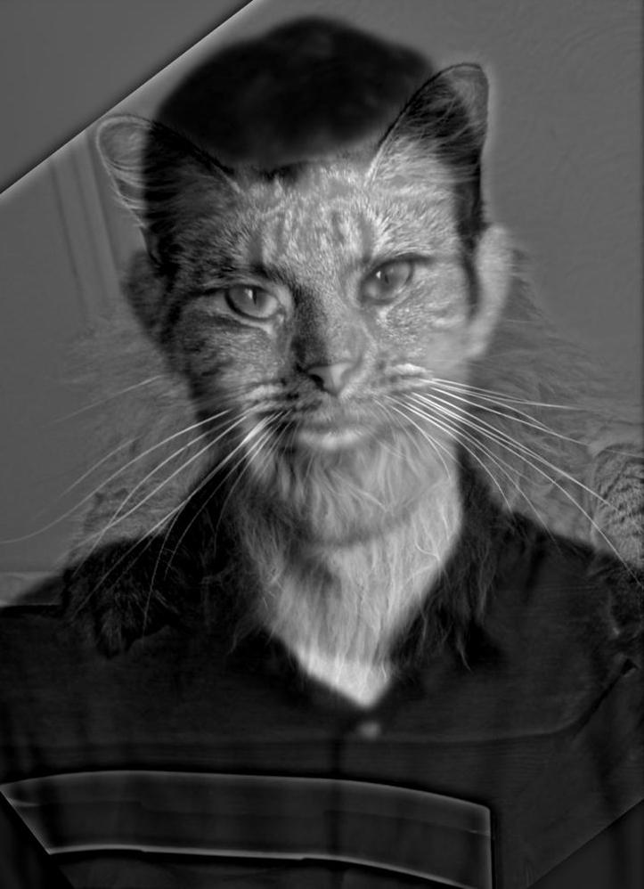
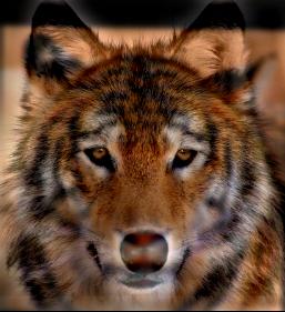 Morph between a tiger and a wolf. |
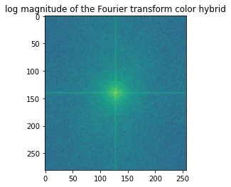 Log magnitude of the Fourier transform for this image. |
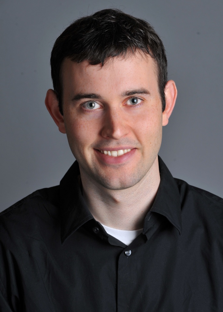
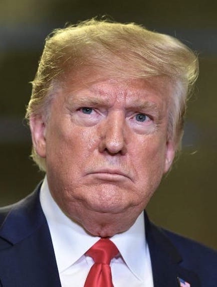
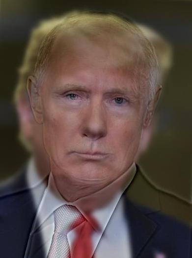
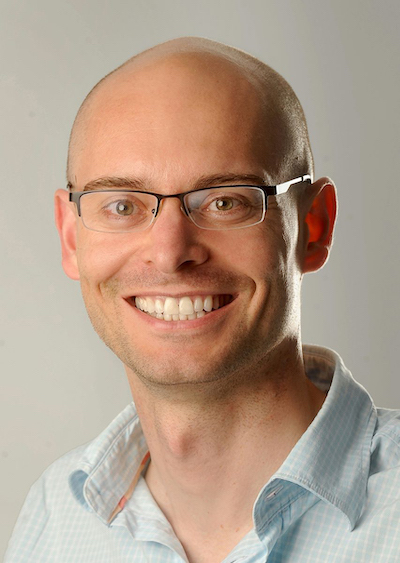
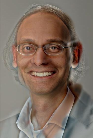
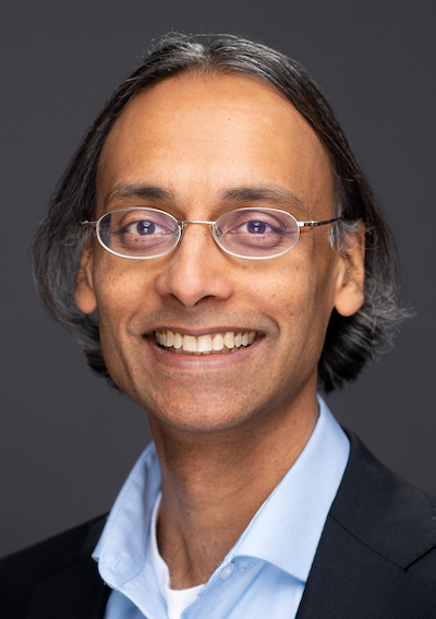
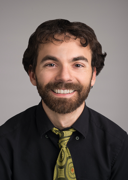
Now, we present some interesting face morphing images which hopefully appear different depending the viewing distance.
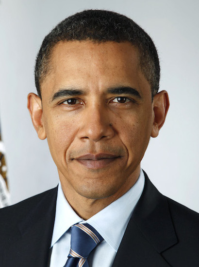 We extract the low frequency from this image. |
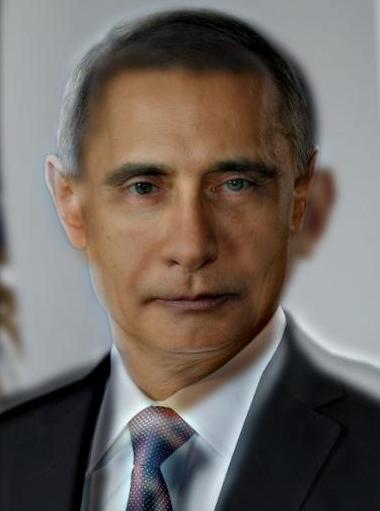 Hybrid Image ksize = 30, Lσ = 4.5, Hσ = 19 |
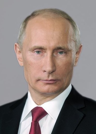 We extract the high frequency from this image. |
||
 We extract the low frequency from this image. |
 Hybrid Image ksize = 30, Lσ = 4.25, Hσ = 3.66 |
We extract the high frequency from this image. |
||
 We extract the low frequency from this image. |
 Hybrid Image ksize = 30, Lσ = 3.55, Hσ = 8.66 |
 We extract the high frequency from this image. |
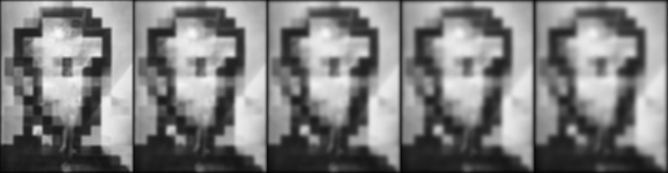
We can simulate a “farther away” view by scaling down the hybrid images. We can observe that the low frequencies are visible while the low frequencies are difficult to discern.
|
|
|
|
|
|
Failure case: If the images to be blended do not share a pretty similar composition, the results won’t be as pleasing as the ones shown above. Blending incompatible images might produce unpleasant and even disturbing results! An example of this is shown below.
 We extract the low frequency from this image. |
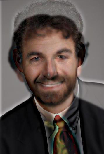 Hybrid Image ksize = 30, Lσ = 2.55, Hσ = 13.6 |
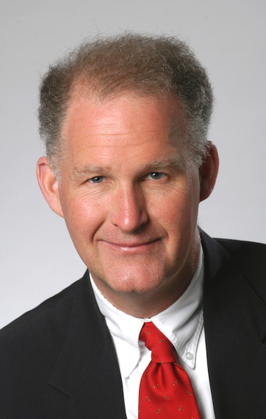 We extract the high frequency from this image. |
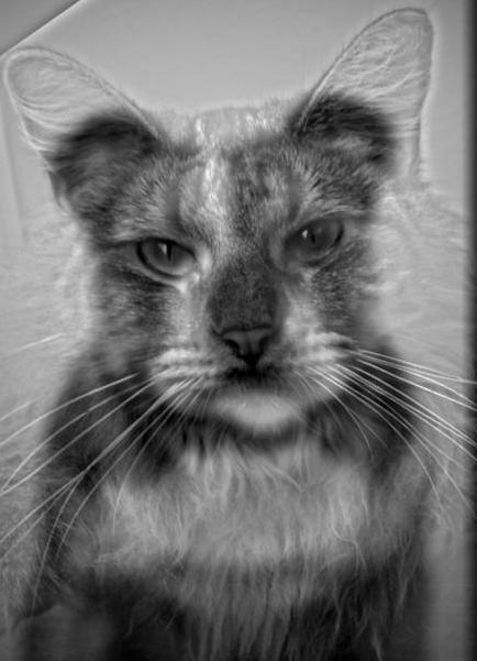
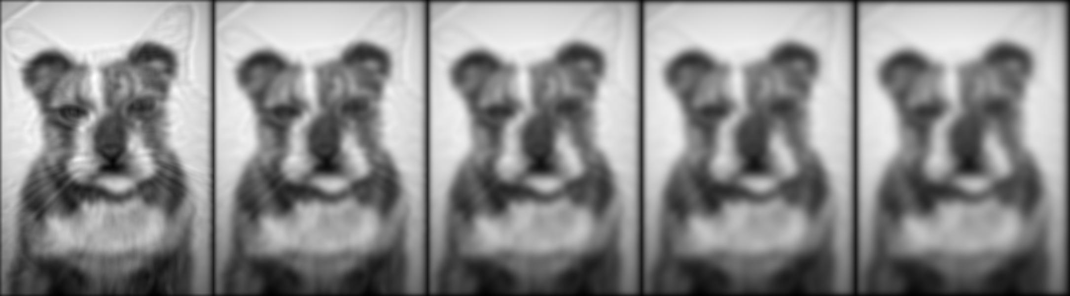
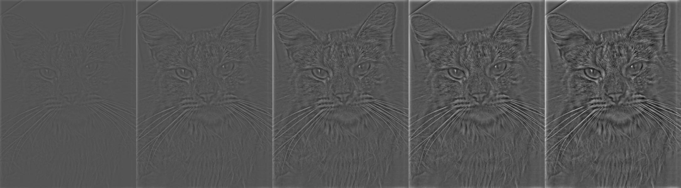
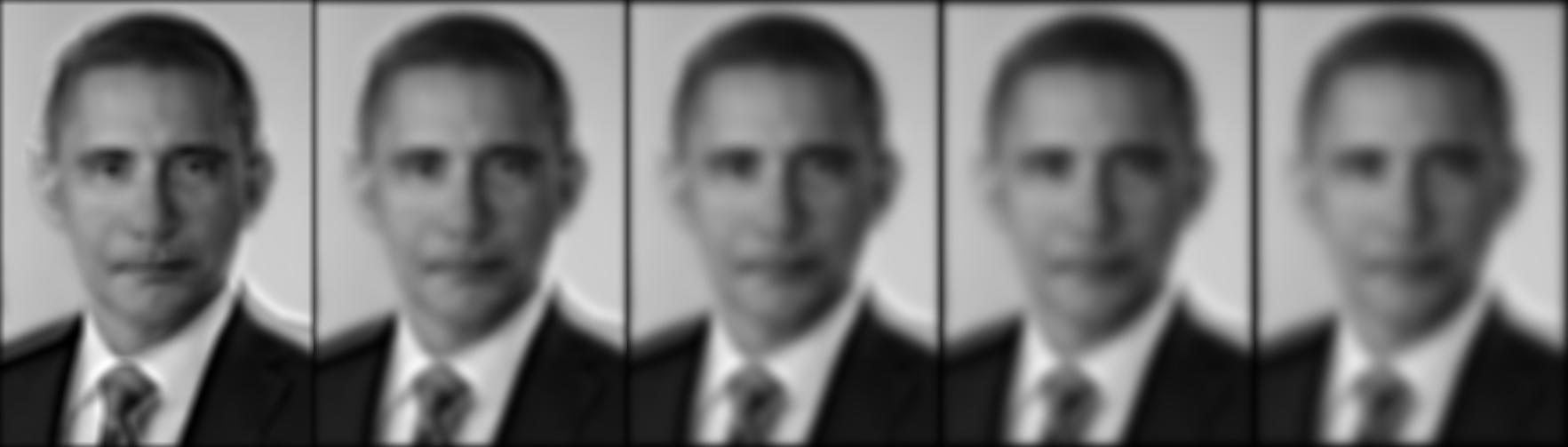
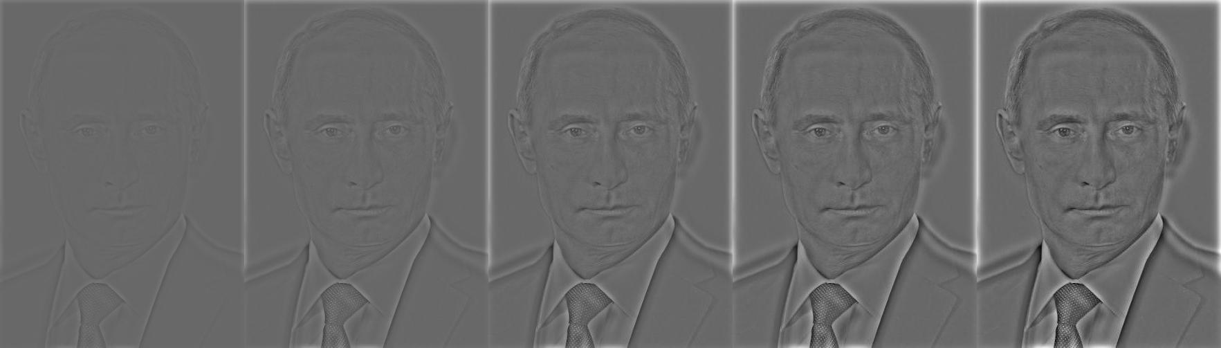
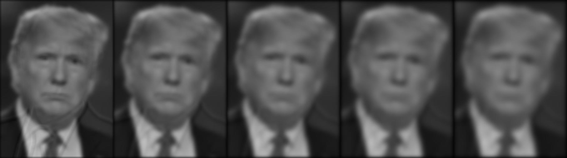
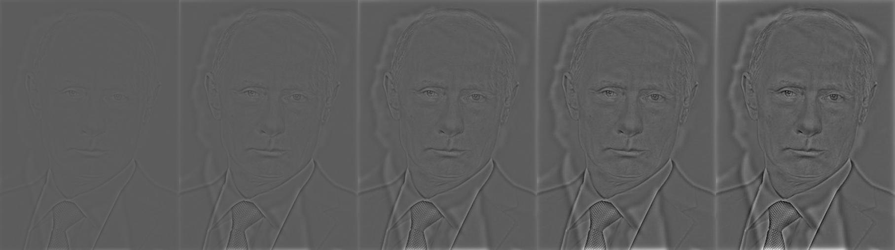
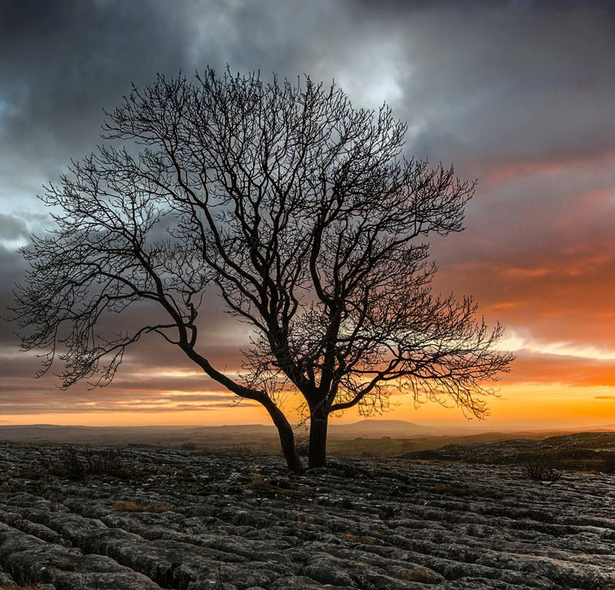
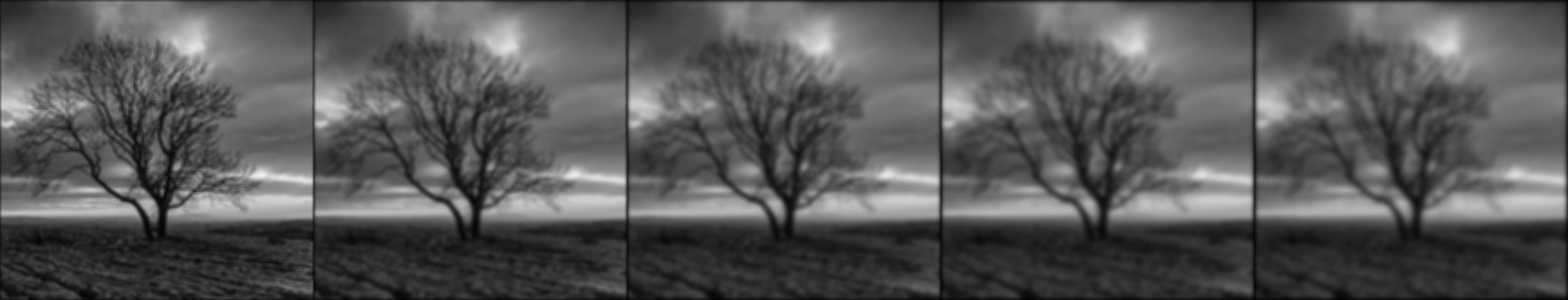
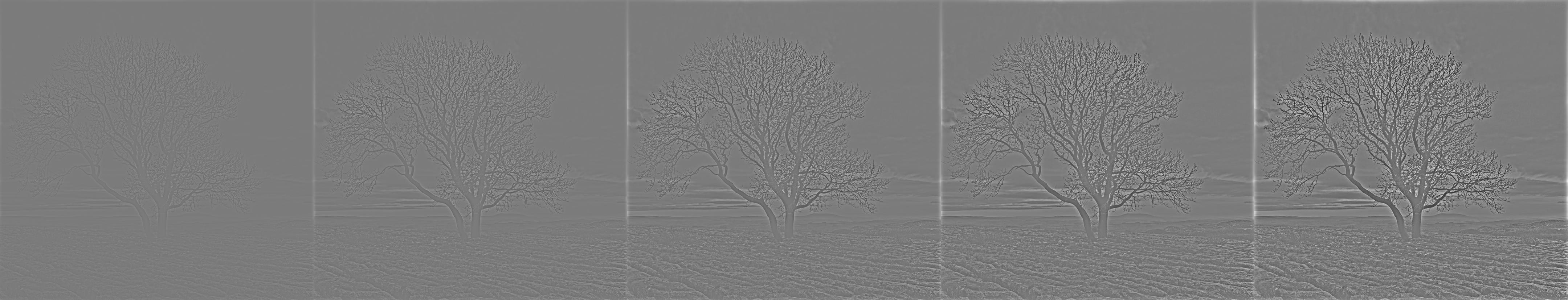
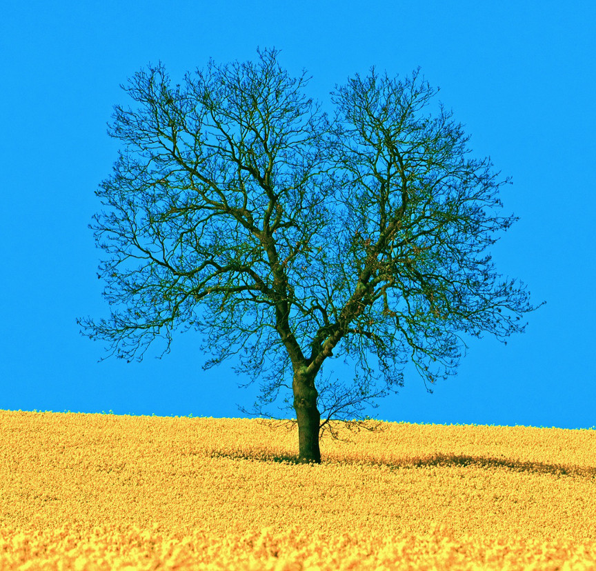
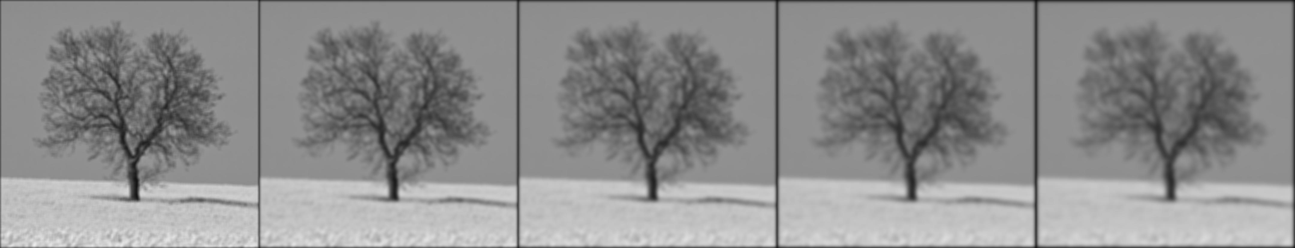
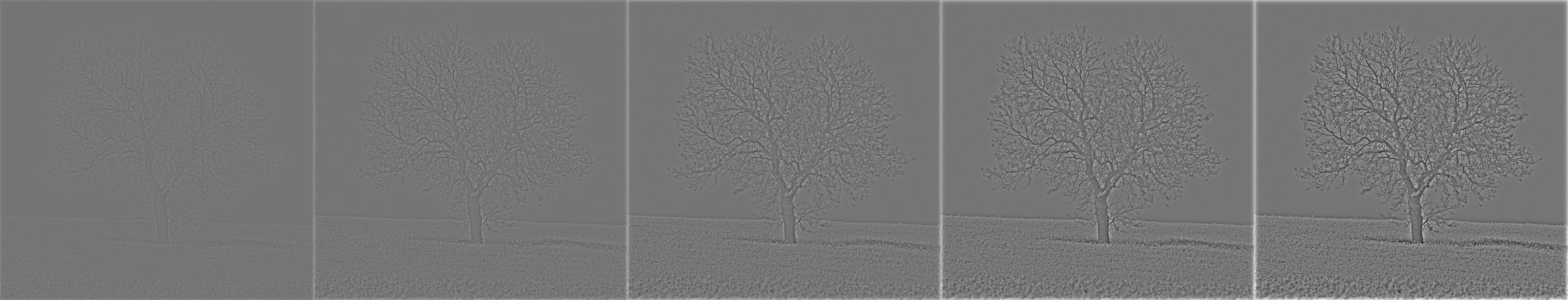
Part 2.3: Gaussian and Laplacian Stacks
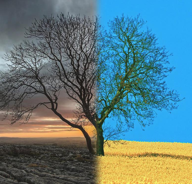
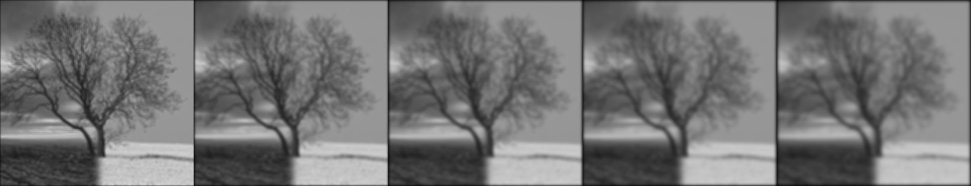
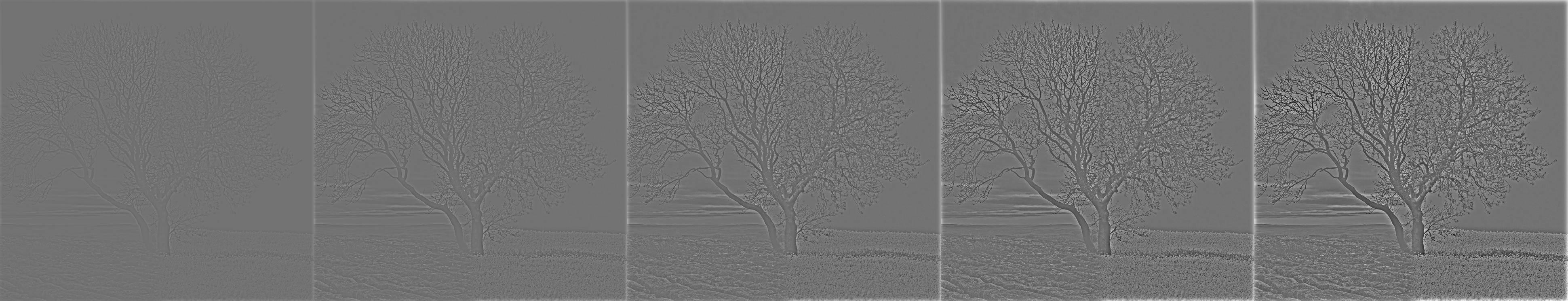
Before we can continue exploring more frequency manipulation applications, we need to build two additional tools that will allow us implementing yet another cool blending application. These new tools are called Gaussian and Laplacian stacks. In a stack the images are never downsampled as in pyramids, so the results are all the same dimension as the original image. To create a Gaussian stack, we just apply the Gaussian filter at each level, so each new layer becomes blurrier (we remove the high frequencies). To create a Laplacian stack, we do follow the same process as for a Gaussian stack, but instead of removing the high frequencies we remove the low frequencies, so all that remains are just the sharp edges of the image. A nice direct application of these stacks is to split the low and high frequencies components from a given image. We show some examples for some hybrid images, including some that we created in the previous part.
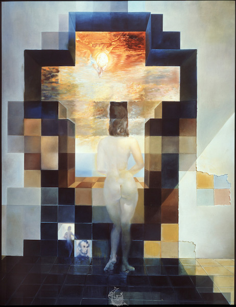 Hybrid image |
 Stack of low frequencies |
|
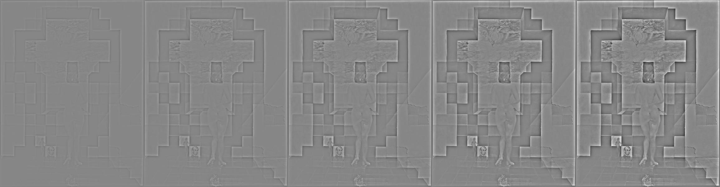 Stack of high frequencies. |
||
 Hybrid image |
 Stack of low frequencies |
|
 Stack of high frequencies. |
||
|
Hybrid image |
 Stack of low frequencies |
|
 Stack of high frequencies. |
||
|
Hybrid image |
 Stack of low frequencies |
|
 Stack of high frequencies. |
Part 2.4: Multiresolution Blending
Finally, we will use our Gaussian and Laplacian stacks to build the Multiresolution Blending Algorithm. The main use of this algorithm is to blend two images seamlessly. In this section, we implement a multiresolution spline technique to combine two or more images into a composed image. This process requires that we first decompose our input images into a set of band-pass filtered component images (Gaussian and Laplacian stacks!). This algorithm can be outlines as follows:
- Build Laplacian stacks LA and LB for images A and B respectively.
- Build a Gaussian stacks GR for the region (mask) image R.
- Form a combined pyramid LS from LA and LB using nodes of GR as weights. That is, for each l, i and j:

- Obtain the splined image S by expanding and summing the levels of LS.
Now we are ready to have some fun again by creating some image blendings! The results are similar to the one we could have obtained from photo edition software such as Photoshop. After all, they may have their basis in some of these core concepts of image manipulation.
 Hybrid image |
 Stack of low frequencies |
|
 Stack of high frequencies. |
||
 Hybrid image |
 Stack of low frequencies |
|
 Stack of high frequencies. |
||
 Hybrid image |
 Stack of low frequencies |
|
 Stack of high frequencies. |
Bells & whistles:
We present some additional examples using color to enhance the effect below.
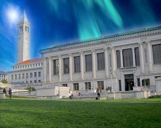
 First image. |
 Second image, |
 White corresponde to first image, black correspond to second image. |
 Blended image |
|||
 First image. |
 Second image, |
 White corresponde to first image, black correspond to second image. |
 Blended image |
|||
|
First image. |
 Second image, |
White corresponde to first image, black correspond to second image. |
 Blended image |
CONCLUSION
Final thoughts
In this project, we surveyed different image manipulation applications that use convolutions with gaussian kernels and other frequency-extraction operations to generate interesting imagery. We demonstrated that images can store plenty of information that can help us to manipulate them in various useful and creative ways. We also learned how our eye plays a role in how we perceive the world around us. Working on the hybrid/morphing image generator was particularly fun since these type of images provide a really interesting visual illusion that depends on the viewing distance. Overall, this project was enriching, challenging, and fun!
 |