Report
Part 1: Fun with Filters
Part 1.1: Finite Difference Operator
This part illustrated how to find the partial derivatives of an image using convolution and the difference operators D_x and D_y. As you can see from the image, the resulting gradient magnitude image is very noisy due to the noise in the picture, leading to poor edges.
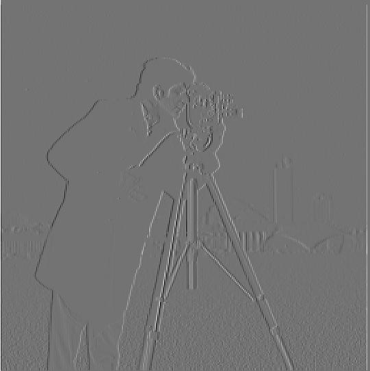 Derivative with respect to x
|
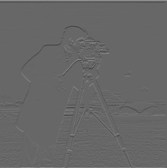 Derivative with respect to y
|
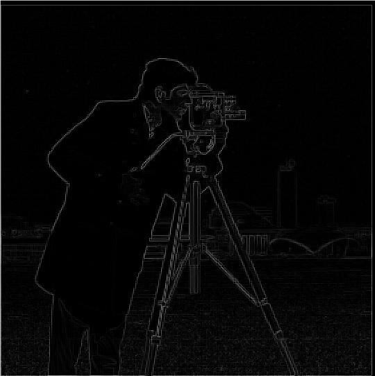 Noisy gradient magnitude
|
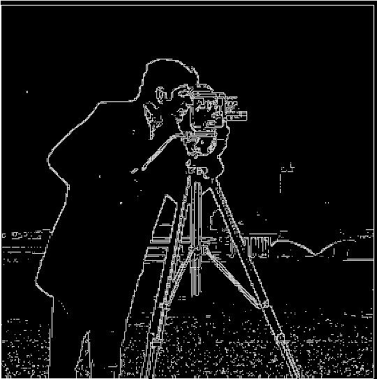 Noisy binarized image
|
Part 1.2: Derivative of Gaussian Filters
Rather than taking the derivatives of the image to construct the gradient magnitude, we instead create the derivative of Gaussian filter in order to eliminate the noise as we compute the gradient. The result is a gradient magnitude with a lot less noise and much smoother edges.
 Derivative of Gaussian with respect to x
|
 Derivative of Gaussian with respect to y
|
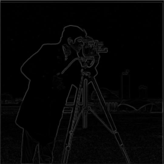 Derivative of Gaussian gradient magnitude
|
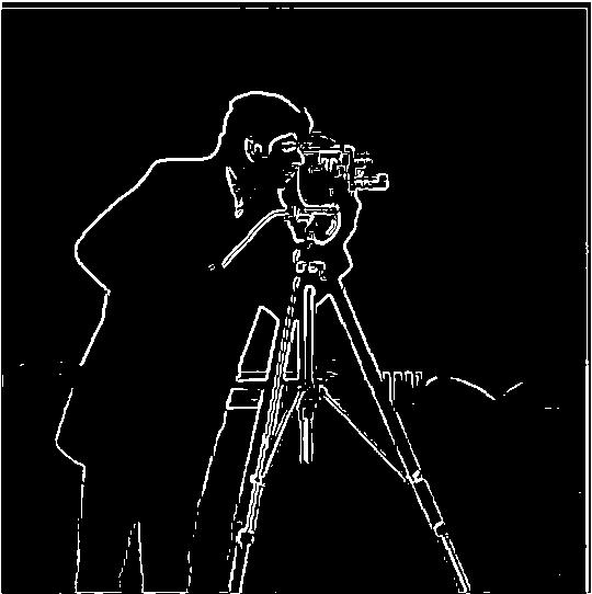 Binarized image with noise removed
|
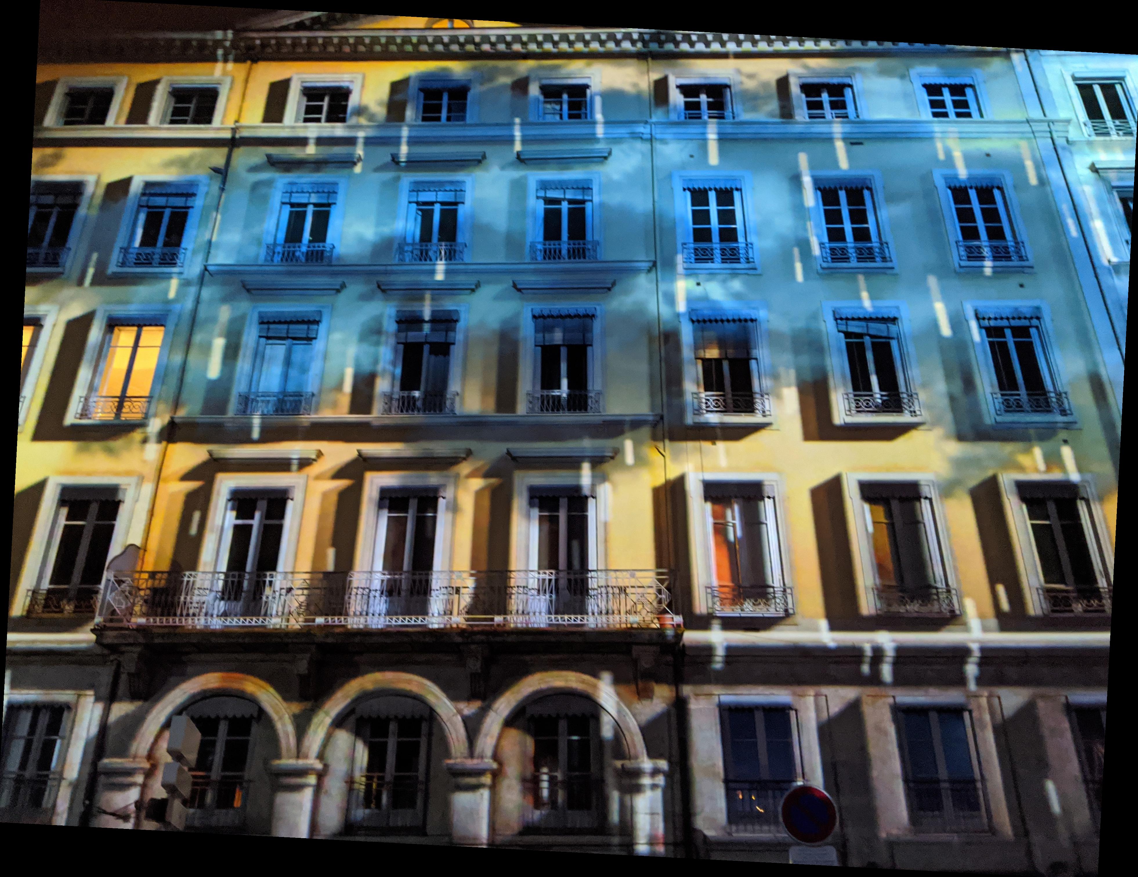
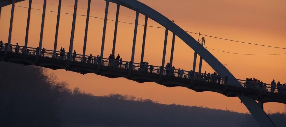
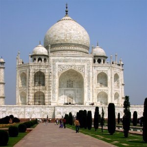
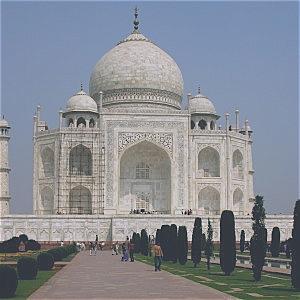
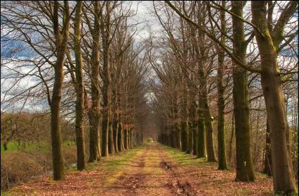
Part 1.3: Image Straightening
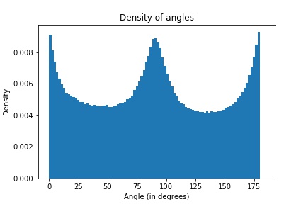
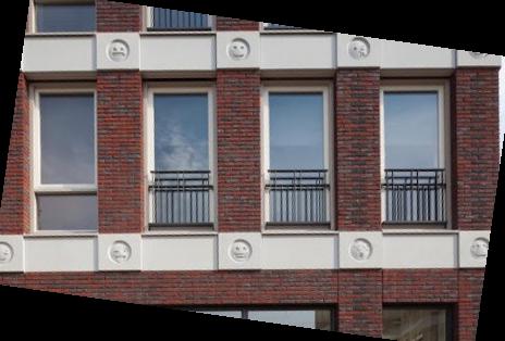
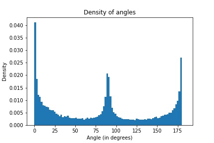
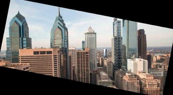
In order to straighten images, we select a set of angles to rotate by. My algorithm chooses rotations from the range [-20, 20). The idea is, we rotate by each angle in our set, crop it to remove the artefacts created from rotation, then calculate the angles of the rotated image. From these angles, we create a histogram, and select the bins that are close to 0, 90, and 180 degrees and sum the proportion of these, selecting the rotation that has the greatest proportion of vertical and horizontal edges.
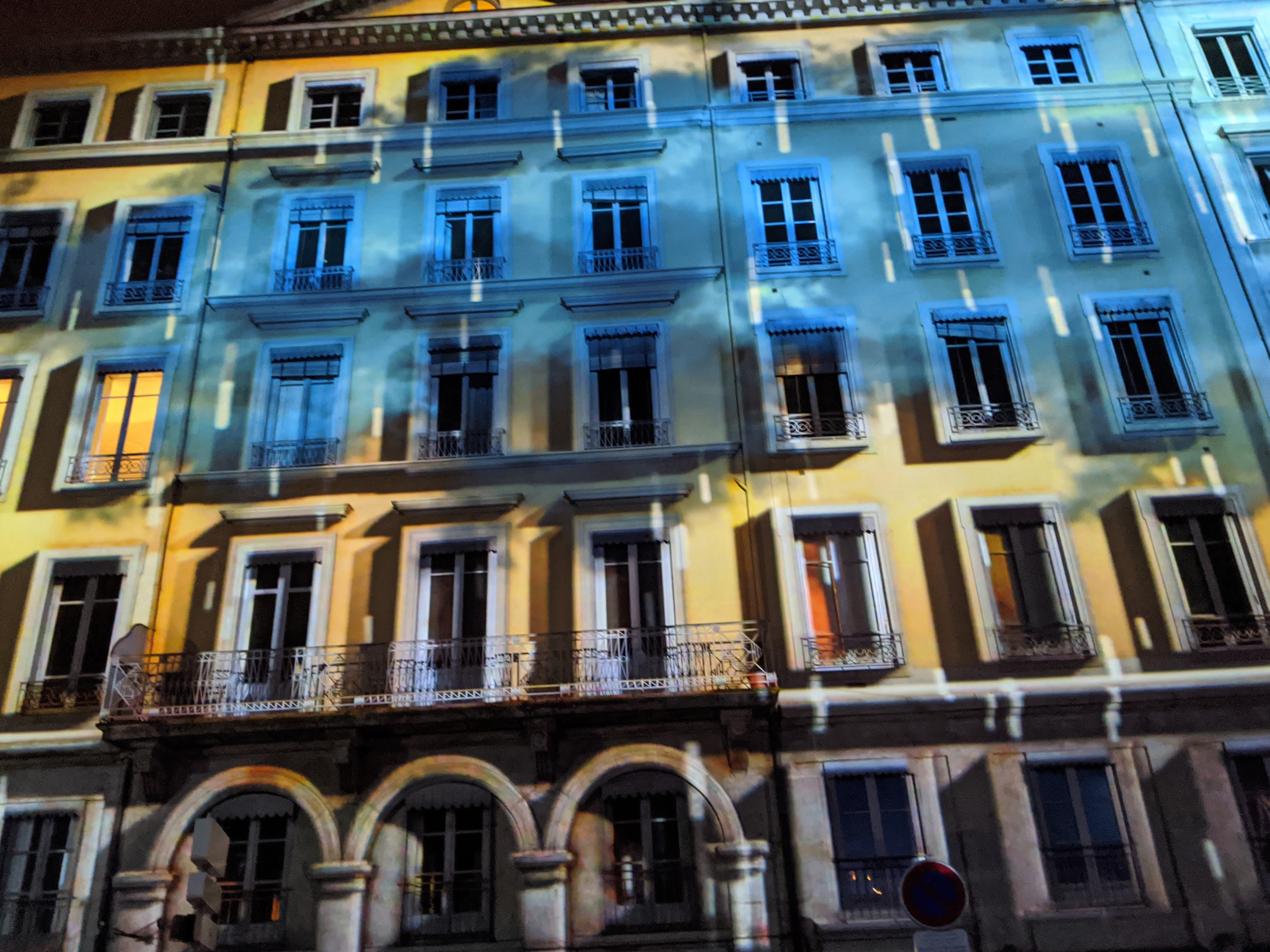 Original, unstraightened image
|
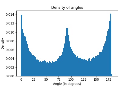
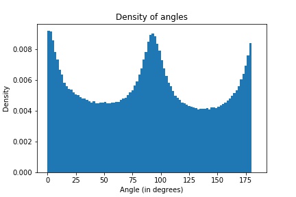 Histogram of edge orientations (in degrees)
|
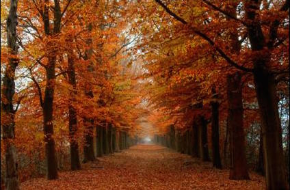
 Straightened image
|
 Histogram of edge orientations (in degrees)
|
 Original, unstraightened image
|
 Histogram of edge orientations (in degrees)
|
 Straightened image
|
 Histogram of edge orientations (in degrees)
|
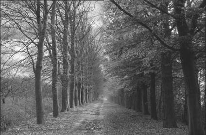
 Original, unstraightened image
|
 Histogram of edge orientations (in degrees)
|
 Straightened image
|
 Histogram of edge orientations (in degrees)
|
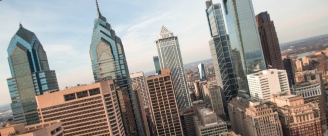
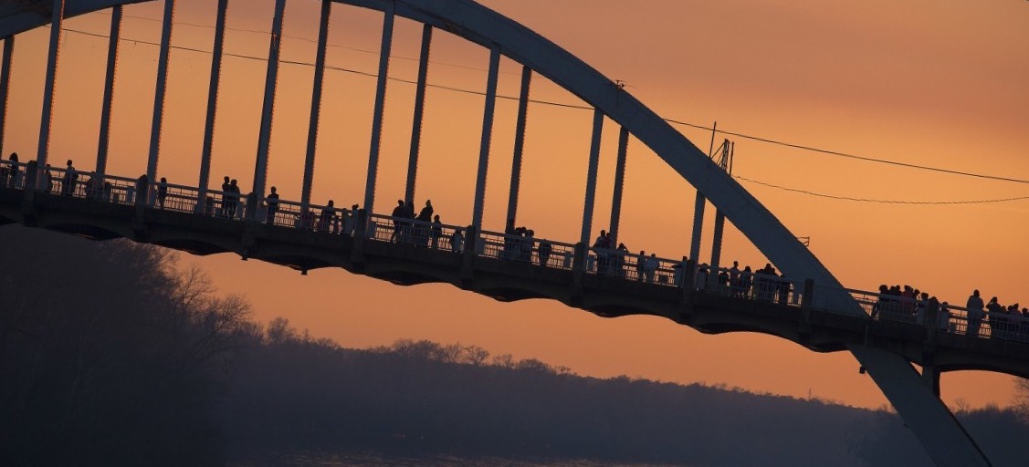 Original, unstraightened image
|
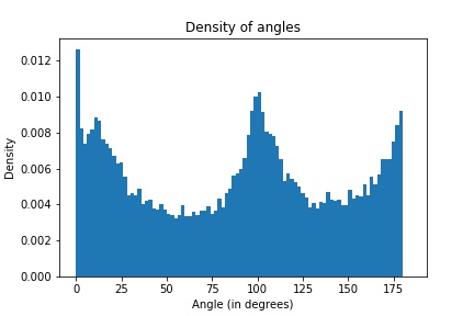
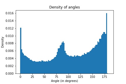 Histogram of edge orientations (in degrees)
|
 Straightened image
|
 Histogram of edge orientations (in degrees)
|
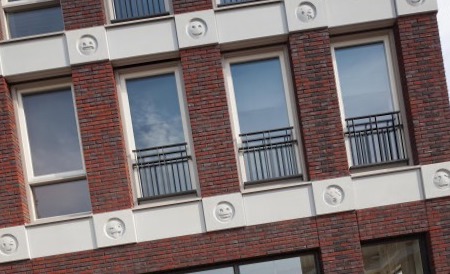
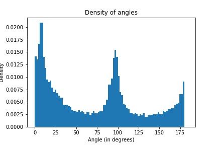
The pair of images above did not straighten properly, and is the failure case of this set. The reason this image straightened so poorly under the algorithm is that the algorithm does not perform well when curved edges are introduced. This image has a large curve throughout the image, making it difficult to find a good rotation since we need an abundant presence of vertical and horizontal edges, not curves.
Part 2: Fun with Frequencies"
Part 2.1: Image "Sharpening"
The main idea of sharpening images is to take a high pass filtered version of an image and add it back to the original image with some weight alpha. To do this in one convolution operation, we construct the Laplacian filter and convolve this with the original image. The Laplacian is created by taking the unit impulse filter, multiplying it by alpha, and then subtracting the Gaussian. This allows us to do one convolution operation to generate a sharpened image.
 Original, unsharpened image
|
 Sharpened image
|
 Original, unsharpened image
|
 Sharpened image
|
In addition, we attempt to restore the original, unsharpened image by taking the sharpened image and blurring it using the Gaussian again. The result is below. As you can see, blurring the sharpened image doesn't quite restore the original image. This is expected since we got the sharpened image through the addition of a high pass filtered image, whereas blurring it simply blurs this sharpened image.
|
Original image
|
 Unsharpened image
|
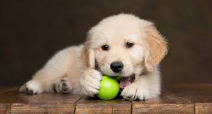
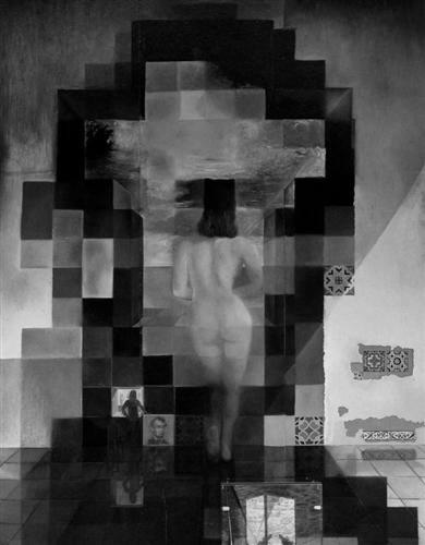
Part 2.2: Hybrid Images
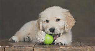
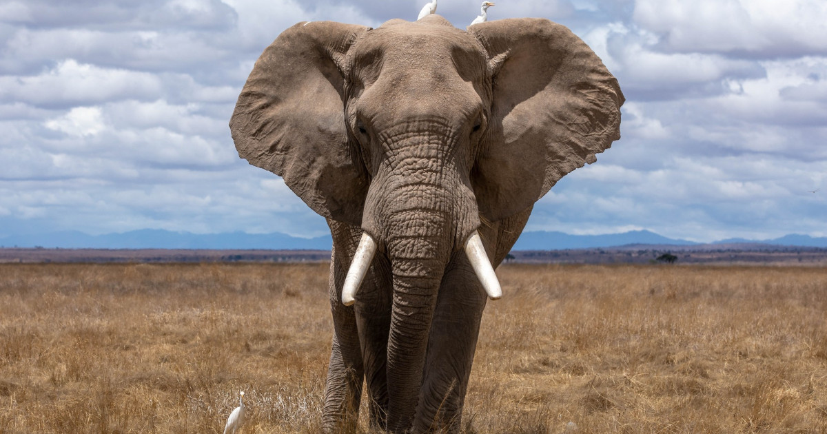
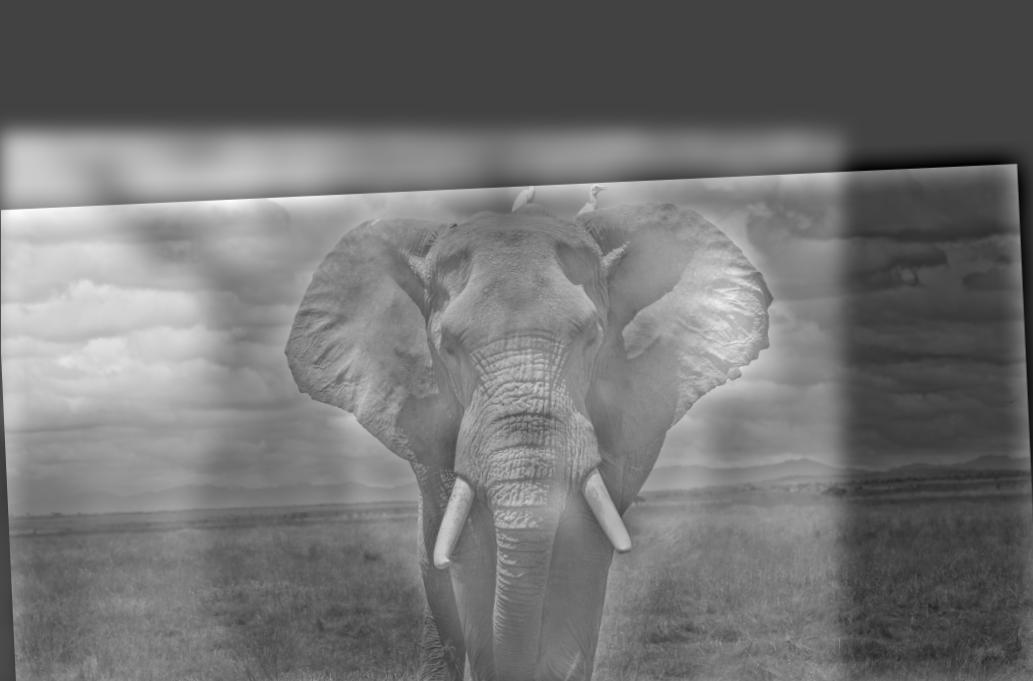
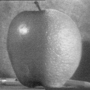
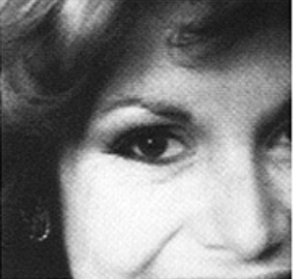
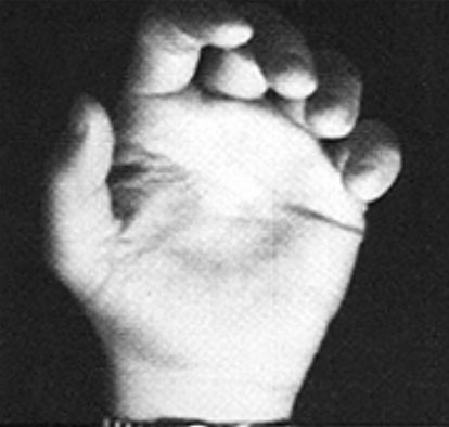
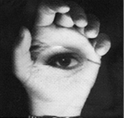
The idea behind creating the hybrid images is to take two images, align them (in the case of these examples, we use the eyes), and compute the high pass filtered version of one and the low pass filtered version of the other. We then combine the two, resulting in an image that shows one image up close at high frequencies and the other image far away at lower frequencies.
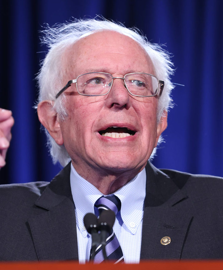
 The image to be seen at low frequencies
|
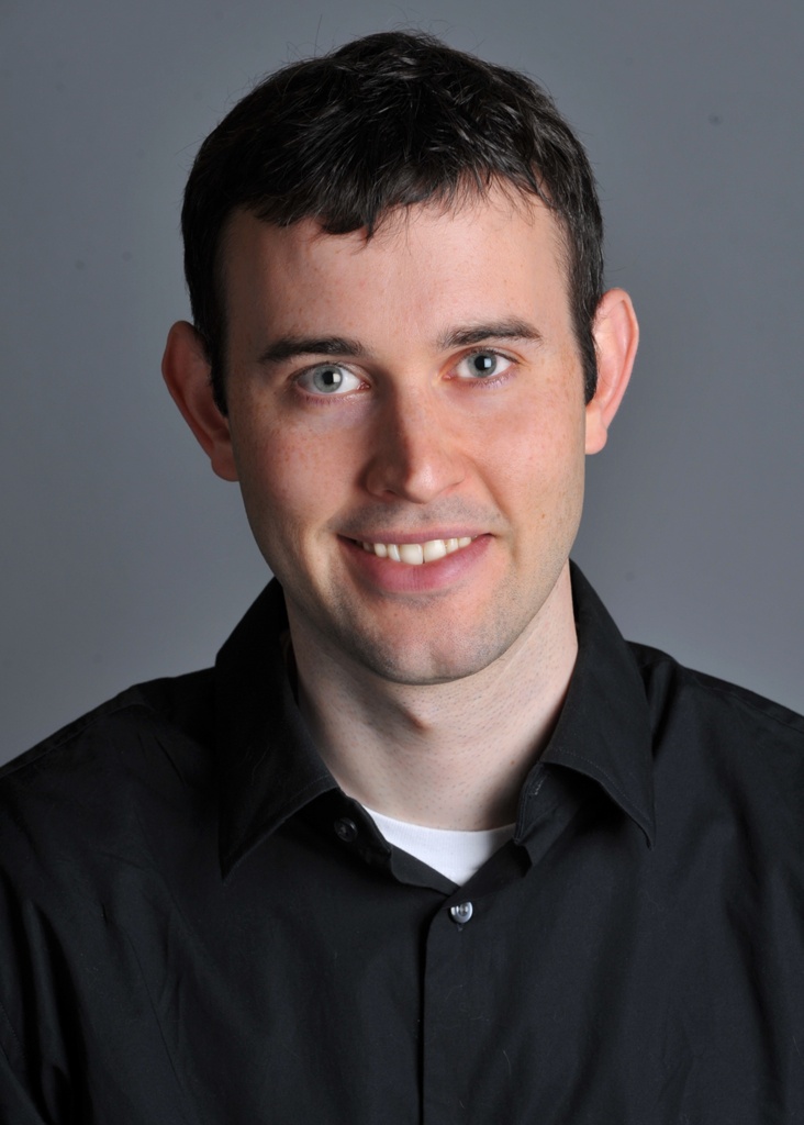
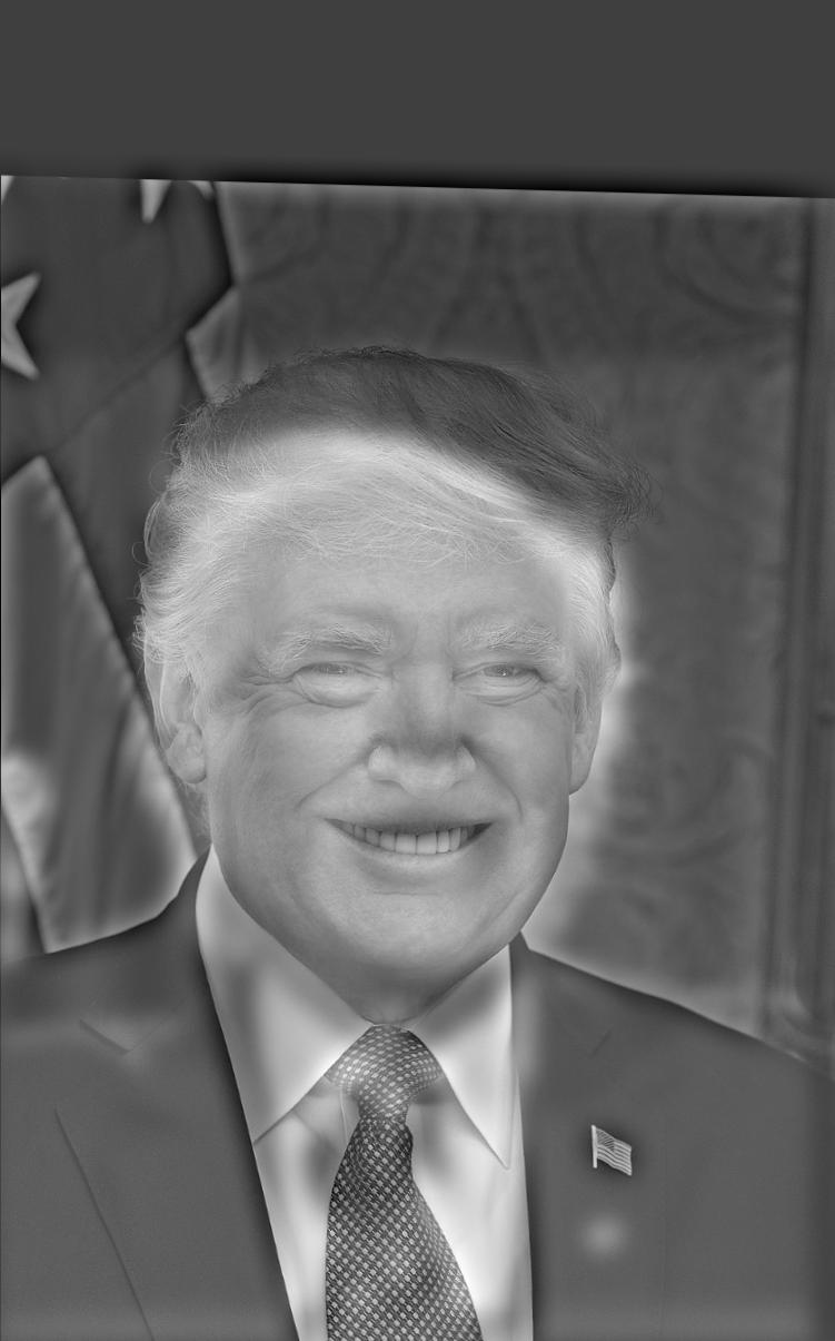
 The image to be seen at high frequencies
|
 The hybrid image
|
 The image to be seen at low frequencies
|
 The image to be seen at high frequencies
|
 The hybrid image
|
 The image to be seen at low frequencies
|
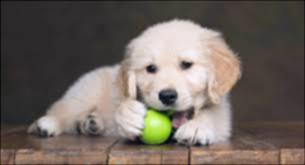
 The image to be seen at high frequencies
|
 The hybrid image
|
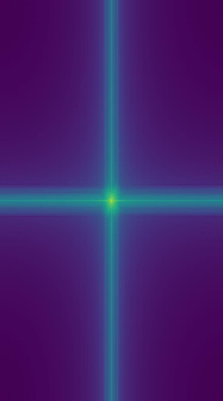
Fourier of DerekPicture.jpg and nutmeg.jpg
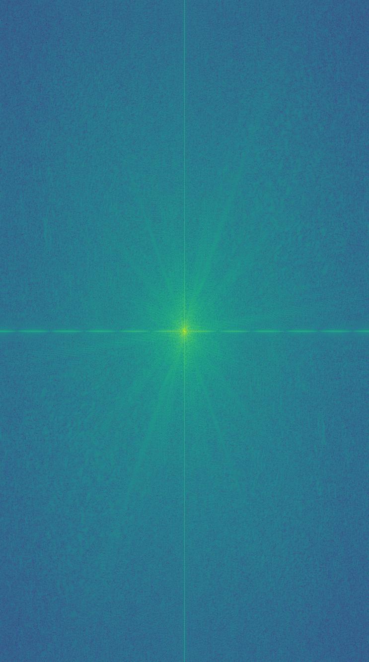 Fourier of image 1
|
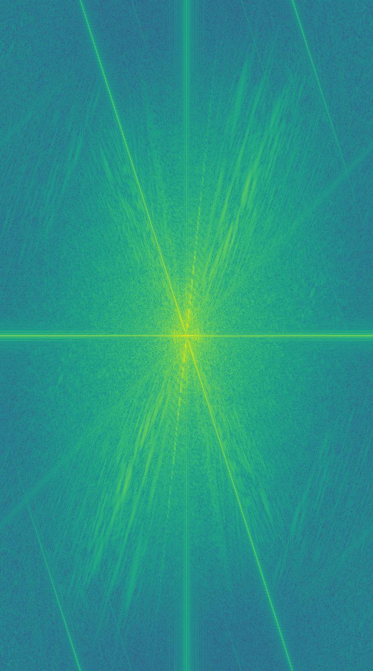
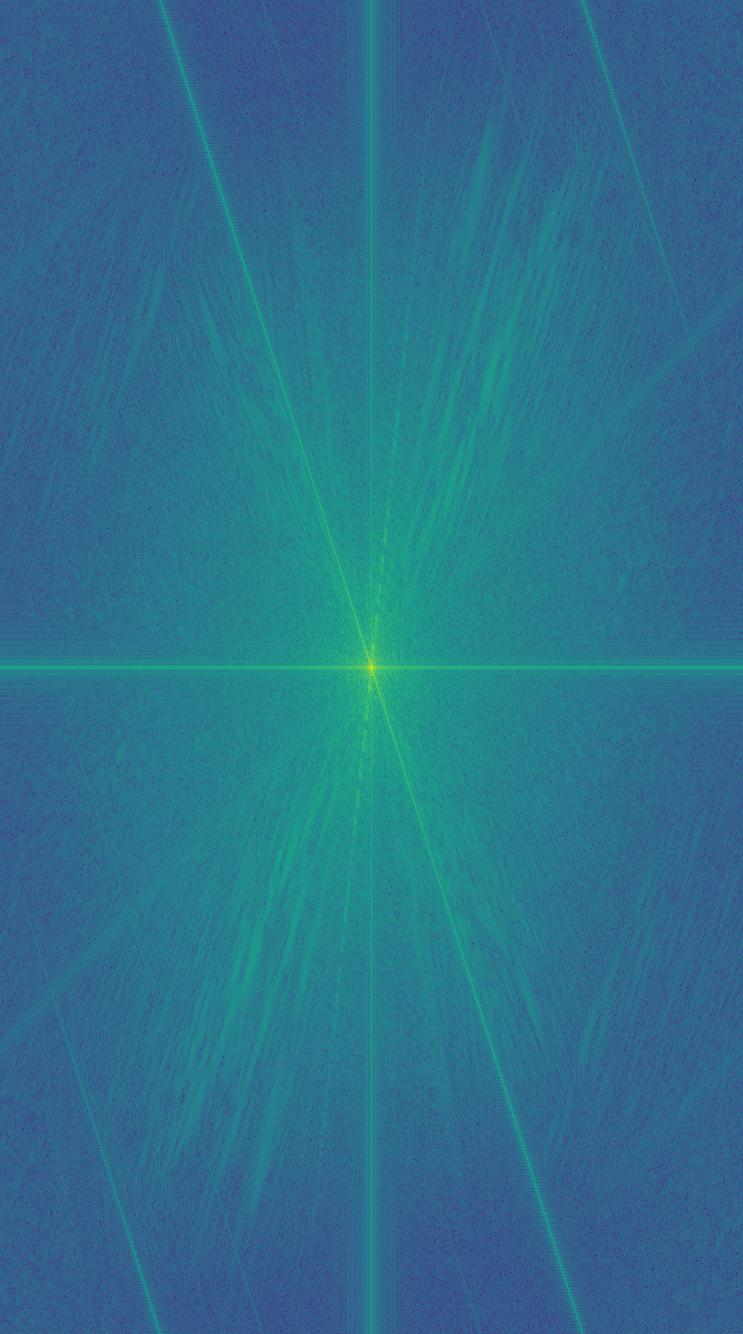 Fourier of image 2
|
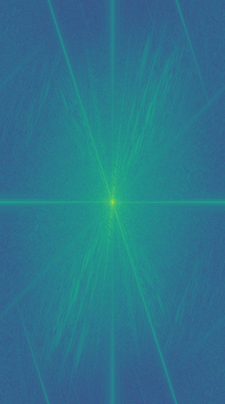
 Fourier of low pass image
|
 Fourier of high pass image
|
 Fourier of hybrid image
|
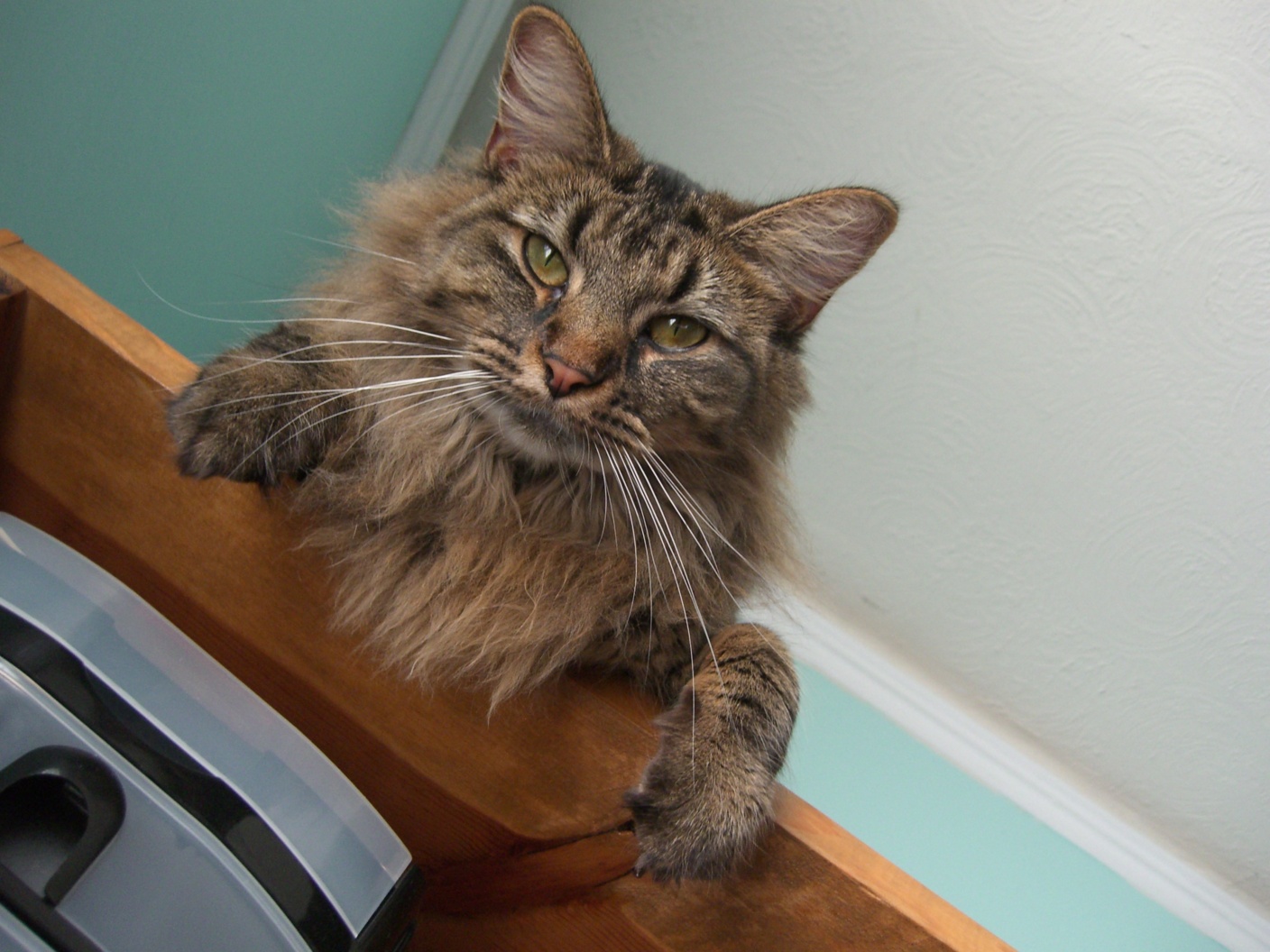
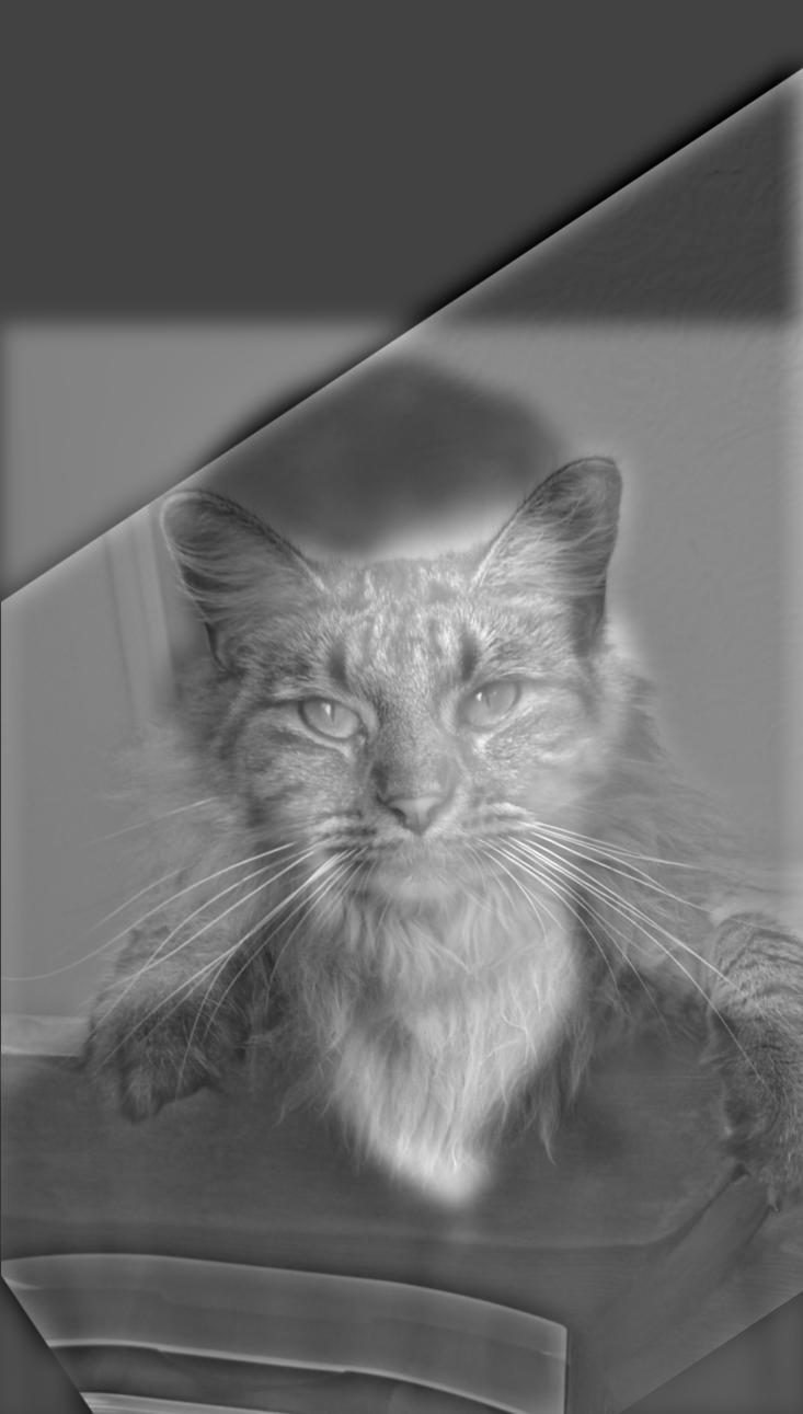
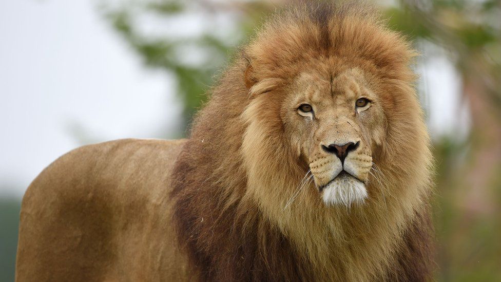
The last set of hybrid images is a failure case as they did not combine together in a nice way. This is because the two images have very different colors and textures, as well as sizing. The images work against each other, with the dark gray vs the bright brown. As a result, this one is much harder to visualize.
Part 2.3: Gaussian and Laplacian Stacks
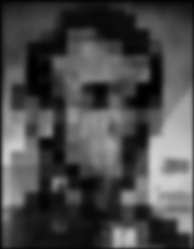
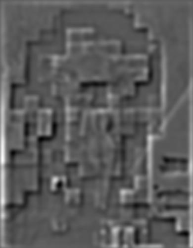
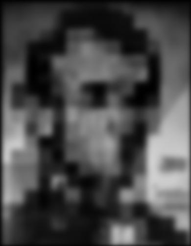
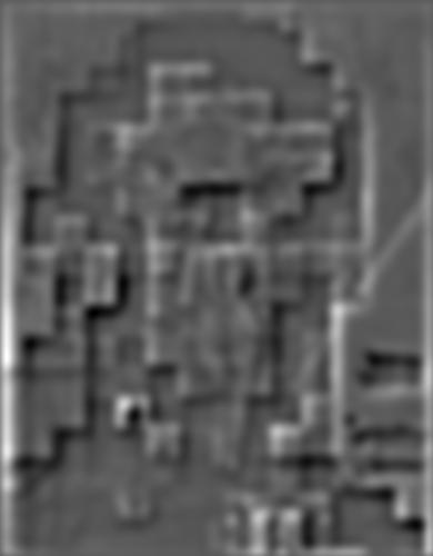
The idea behind creating the Gaussian stacks is to repeatedly apply a Gaussian to an image to blur it down and down until the level we want. The result is a stack of progressively blurred images where we can see the different stages of lower frequencies. To create the Laplacian, we take a pair of Gaussians and subtract them to create high pass images of higher frequencies at each level. Keep in mind there will always be 1 less Laplacian layer than the Gaussian since we rely on the next level Gaussian to generate the Laplacian.
Lincoln Stacks
 Level 0 of Gaussian stack
|
 Level 0 of Laplacian Stack
|
 Level 1 of Gaussian stack
|
 Level 1 of Laplacian Stack
|
 Level 2 of Gaussian stack
|
 Level 2 of Laplacian Stack
|
 Level 3 of Gaussian stack
|
 Level 3 of Laplacian Stack
|
 Level 4 of Gaussian stack
|
 Level 4 of Laplacian Stack
|
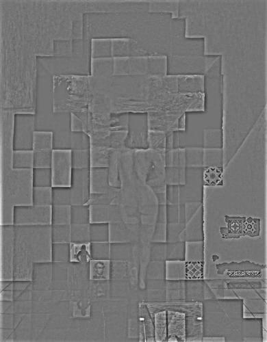
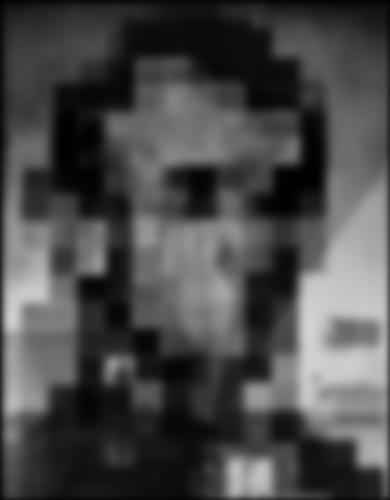
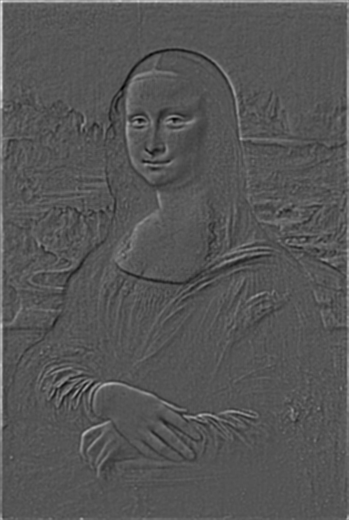
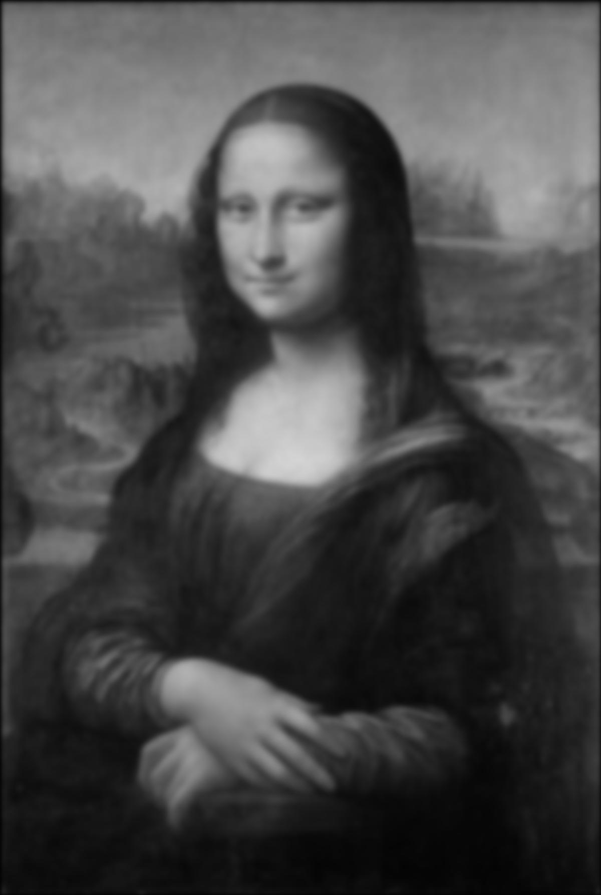
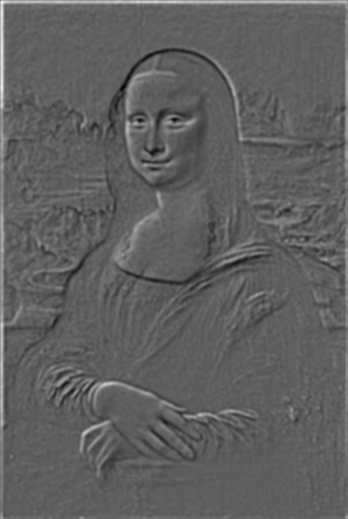
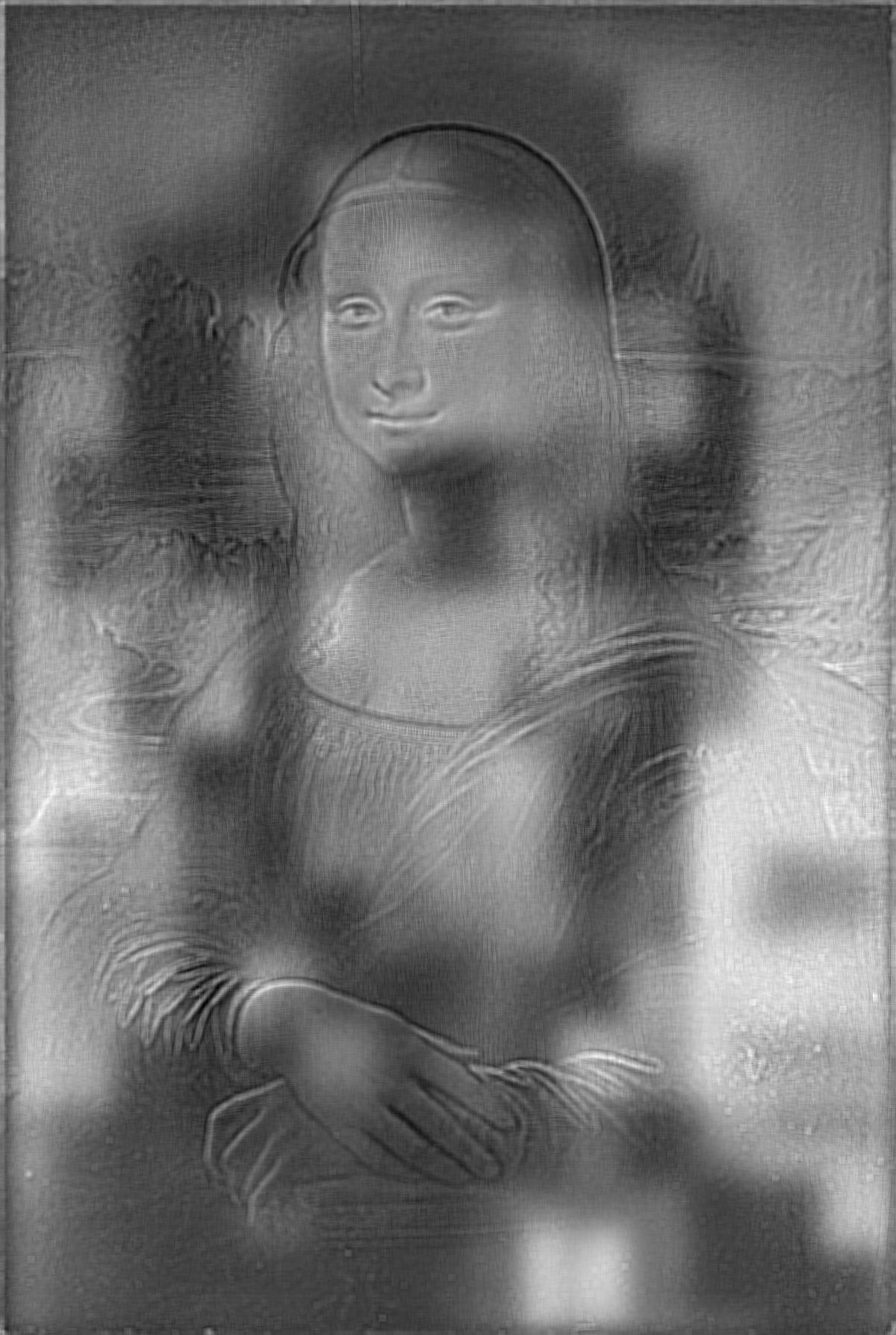
Mona Lisa Stacks
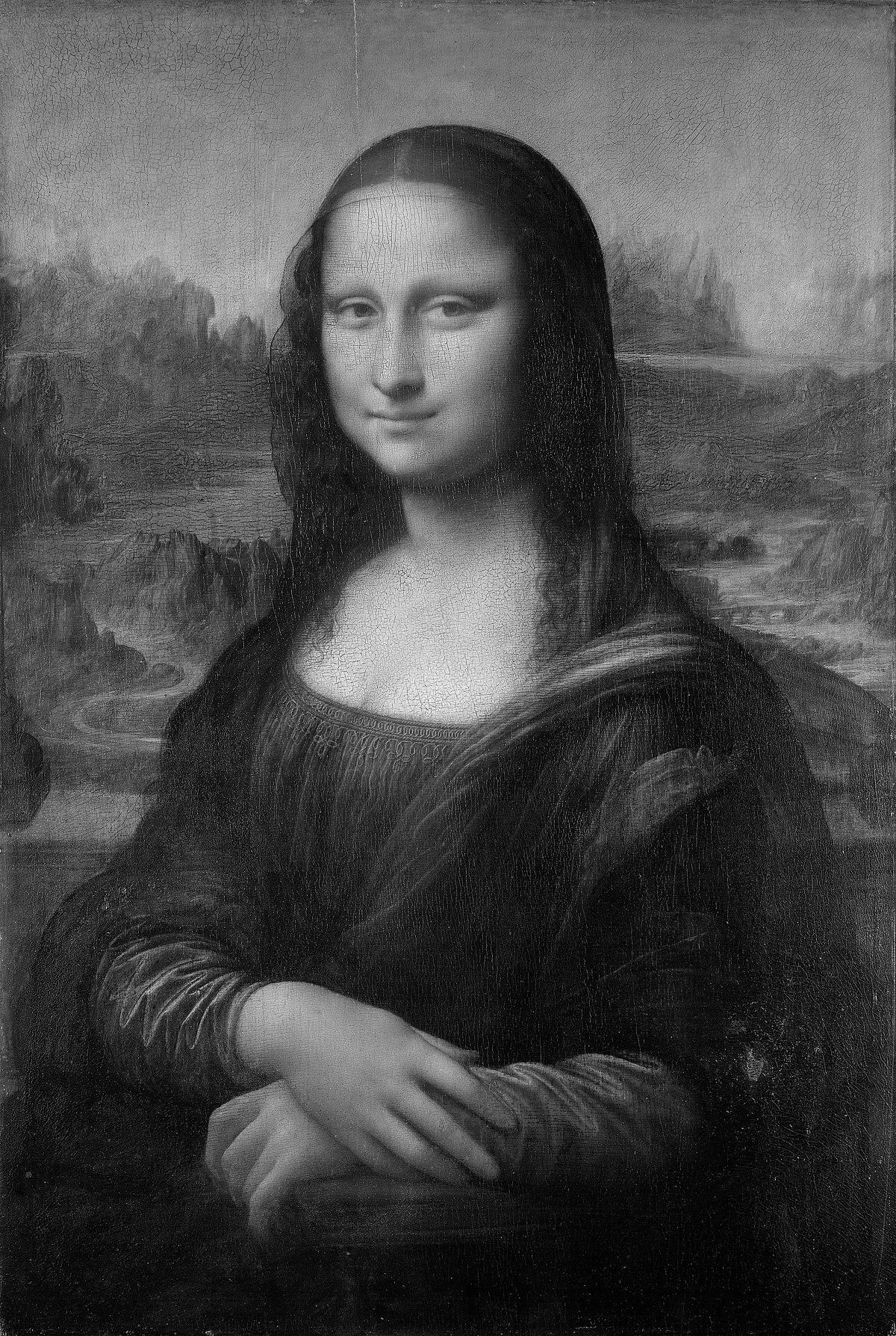 Level 0 of Gaussian stack
|
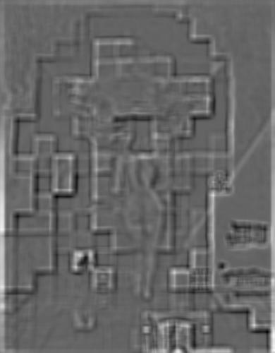
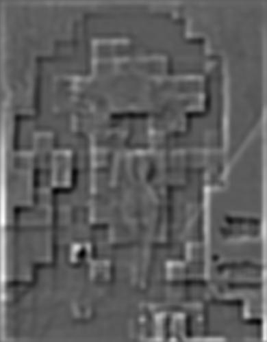
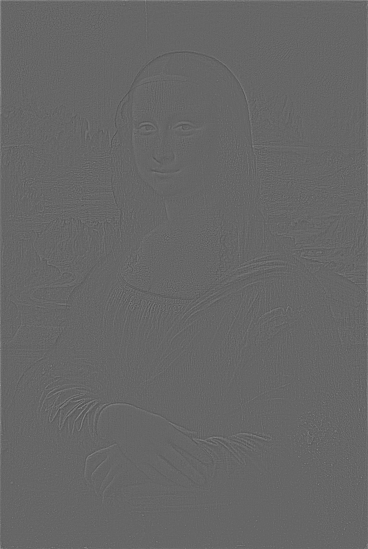 Level 0 of Laplacian Stack
|
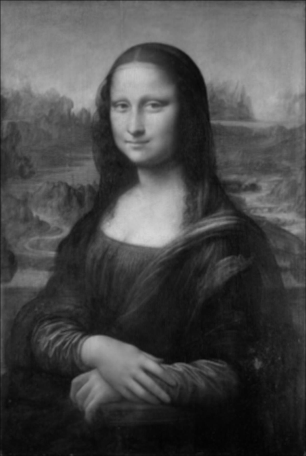 Level 1 of Gaussian stack
|
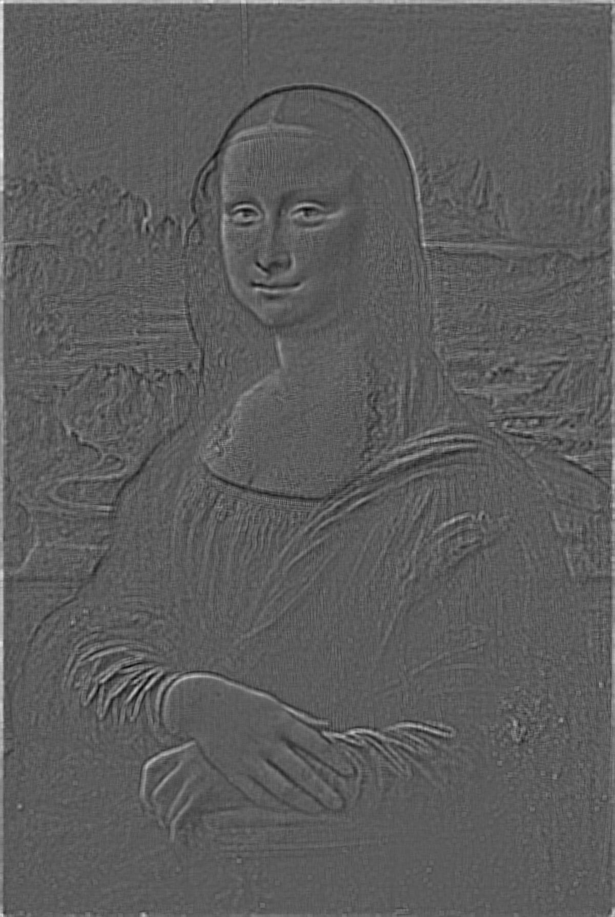 Level 1 of Laplacian Stack
|
 Level 2 of Gaussian stack
|
 Level 2 of Laplacian Stack
|
 Level 3 of Gaussian stack
|
 Level 3 of Laplacian Stack
|
 Level 4 of Gaussian stack
|
 Level 4 of Laplacian Stack
|
Hybrid images from stacks
We can use the laplcian and gaussian stacks to create a hybrid image since we're using high pass and low pass images. The following is the result:
|
Lincoln Gaussian stack level 4
|
Mona Lisa Laplacian stack level 4
|
 Hybrid image
|
Part 2.4: Multiresolution Blending
The main idea behind image blending is to create a laplacian stack for each image to blend, as well as a gaussian stack for the masked region to blend, blending each level together using the mask and summing them all up at the end (including the last blended level of the gaussian stack for each image)
 First image
|
 Second Image
|
 Blended Image
|
 First image
|
 Second Image
|
 Blended Image
|
 First image
|
 Second Image
|
 Blended Image
|