The task of this project is to colorize the Prokudin-Gorskii photo collection. His photo collection consists of 3 separate color channel images that appear to the normal eye as gray. Our job was to combine these separate color channel images into one colorized image output.
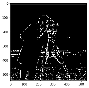
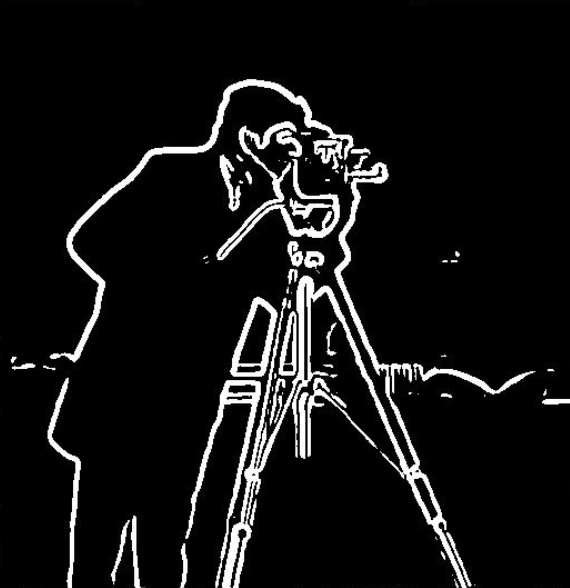
To compute the gradient magnitude image, I calculate the square of the images convolved with the Dx and Dy. Then I added those up and after I took the square root of that. The threshold for this main image is 0.13. As you can see from the image below, there is still plenty of noise at the bottom. But that is where the next part of this project comes in to save the day.
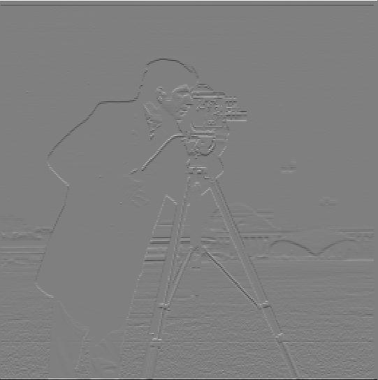
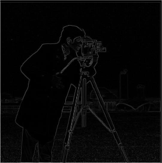
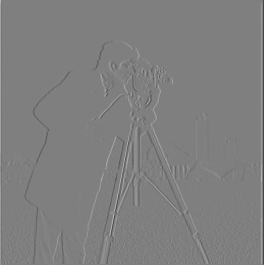
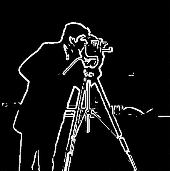
For the first part of this problem, I did what was asked. I blurred the image using the gaussian filter before applying the dx and dy operators. With this resulting image. I noticed it was a lot clearer and less noise than the results from 1.1. However, I also did the second part of the problem to see if I got the same image results when I would convolve the gaussian filter with dx and dy before applying the convolved filters onto the image. I still got the same clear, non noisy results which was very cool as well. I show the two results from both methods below, as well as images of the x gradient filter and the y gradient filter. (Gaussian kernel parameters: ksize = 5, sigma = 2)


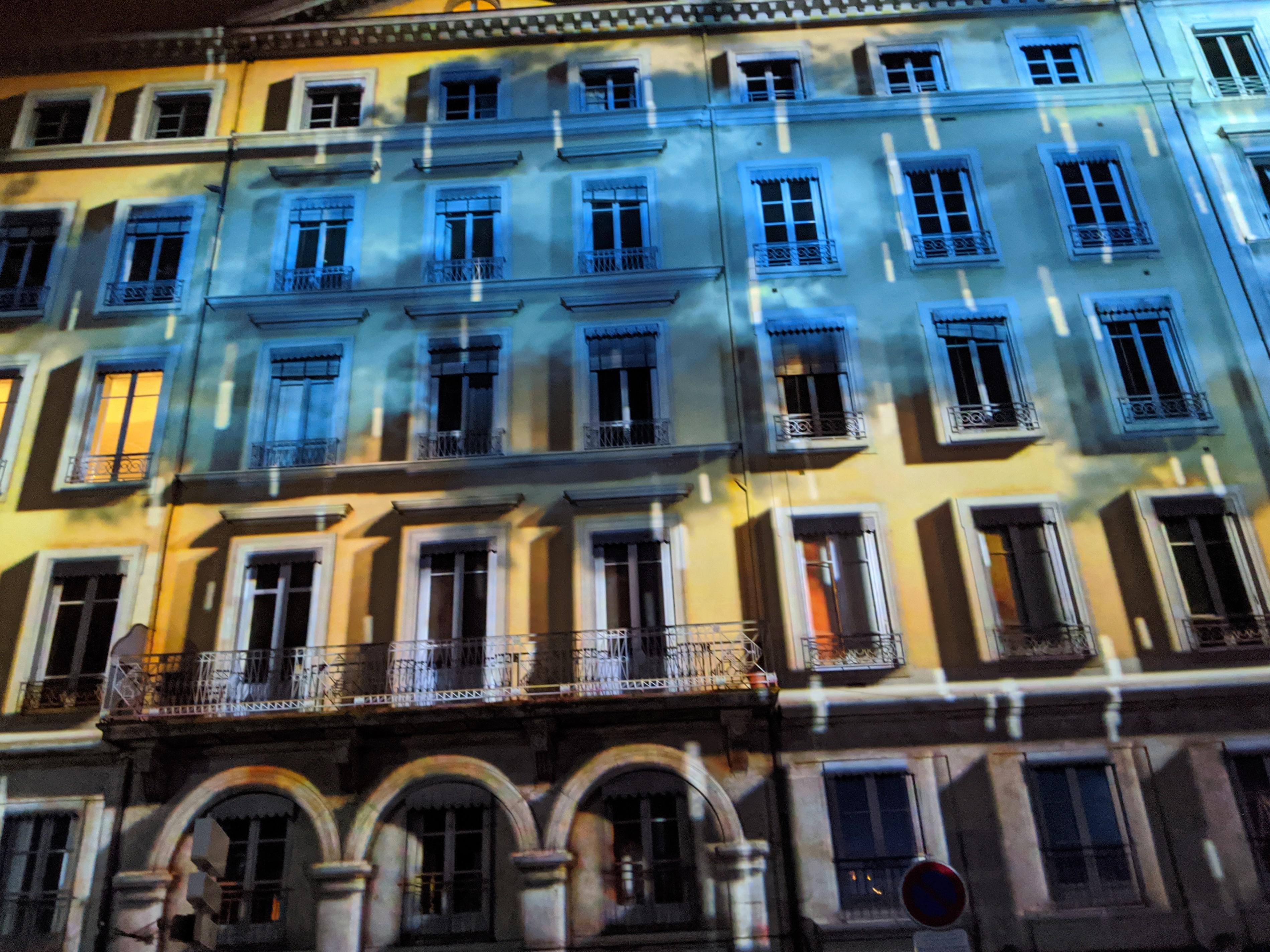
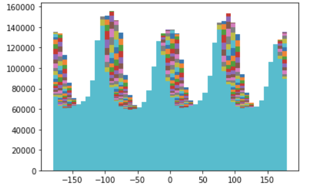
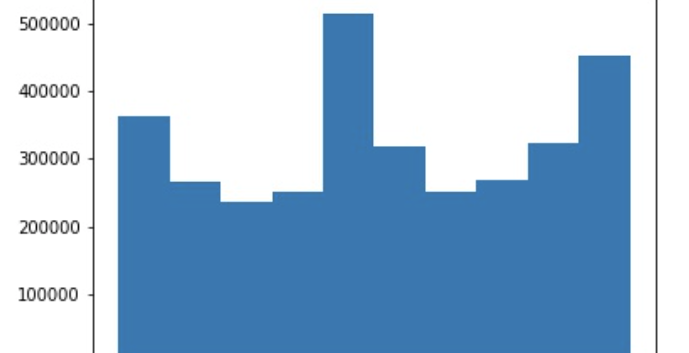
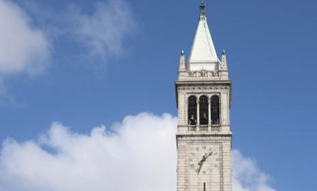
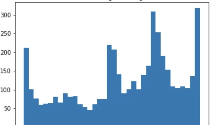
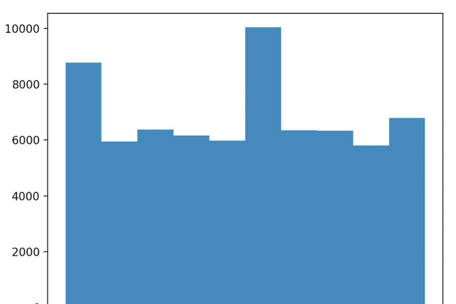
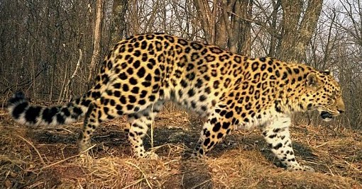
In the final section of part 1, we use what we learned to do automatic rotation to try to achieve a straight image. We learn in this part that images with right angles and straight lines are more likely to be straighter images. We use the derivatives to calculate the gradient angles of an image. We do this by calculating the distribution of gradient angles for each angle rotation between -15 to 15 to determine what the best angle is for a straight image (as shown in my histogram). Our kernal size here is 5 and our sigma is 2
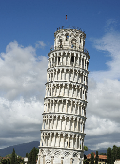
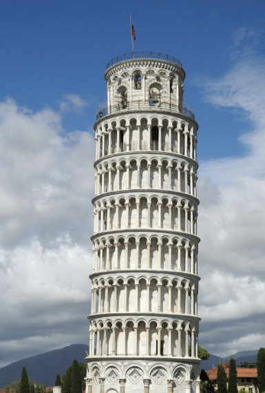
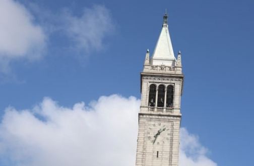
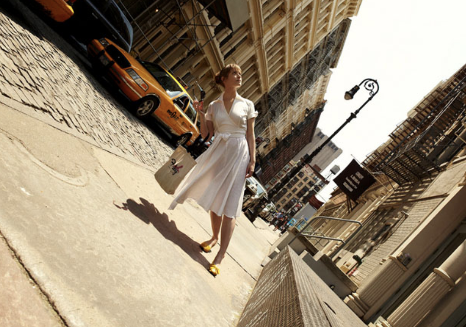
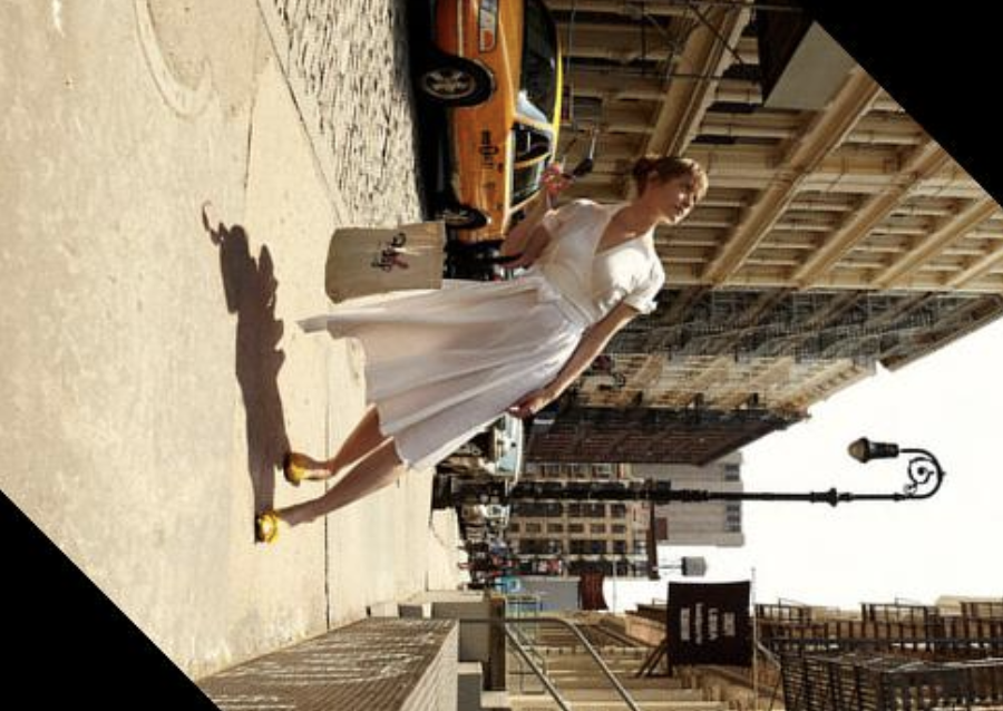
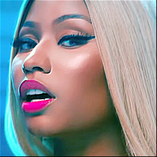
I noticed everyone doing the woman image case and i thought it was interesting so i wanted to find out for myself. Sure enough, it failed with my algorithm. I believe the reason it failed is because my algorithm cannot differentiate between horizontal and vertical lines properly so it ended up orienting her sideways instead of right side up. I thought this was super fascinating!
We then got into making images sharper. Images can be sharpened by by upping the higher frequencies. We do this by first subtracting the blurred image from the original image. This can be put together into a single unsharp filter using a combination of weighted unit impulse function and gaussian filter. Below, I show the original image, sharpened image, and me blurring the image myself.


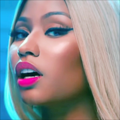
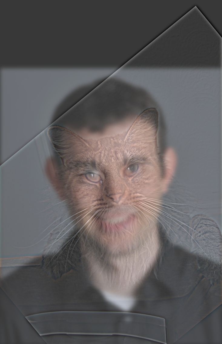
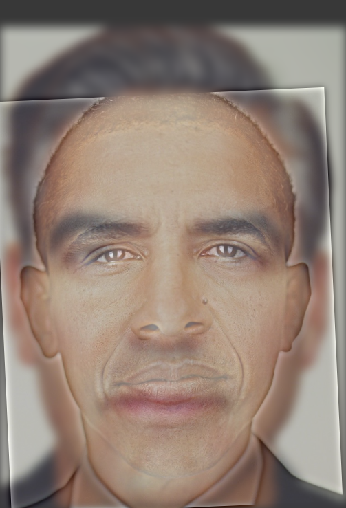
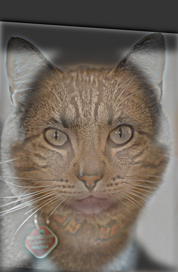
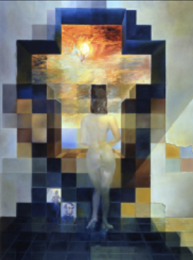
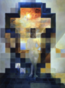
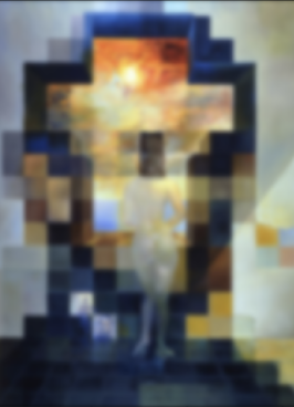
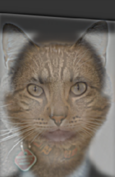
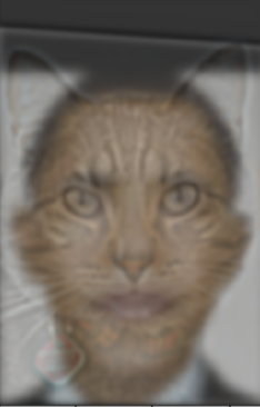
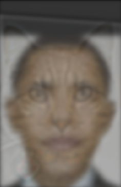
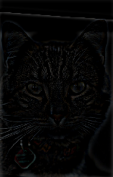
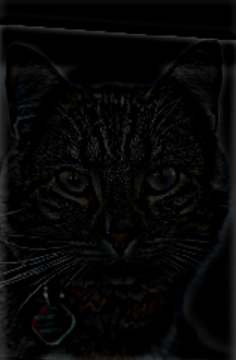
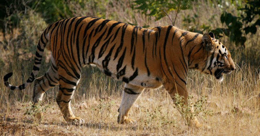
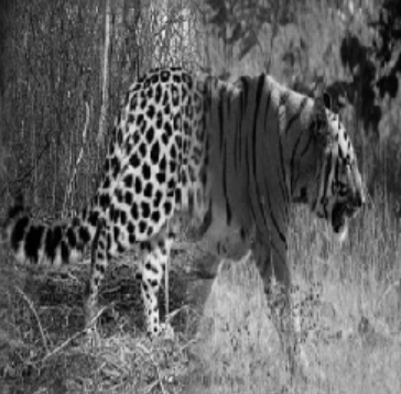
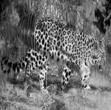
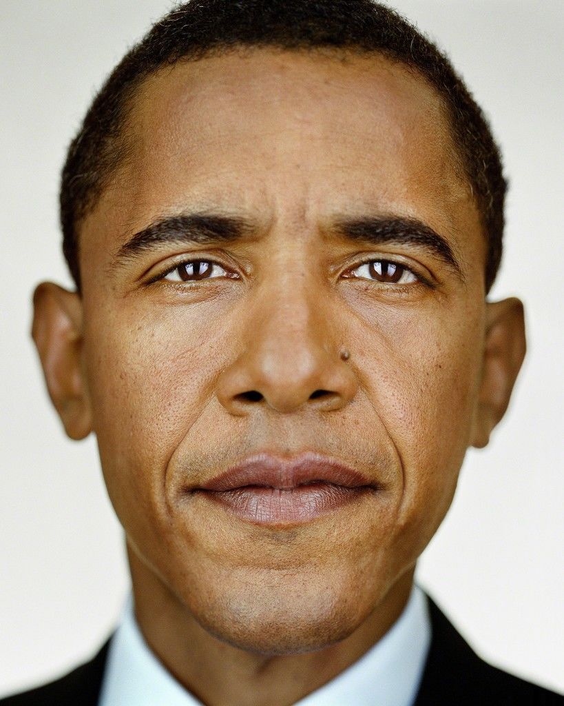
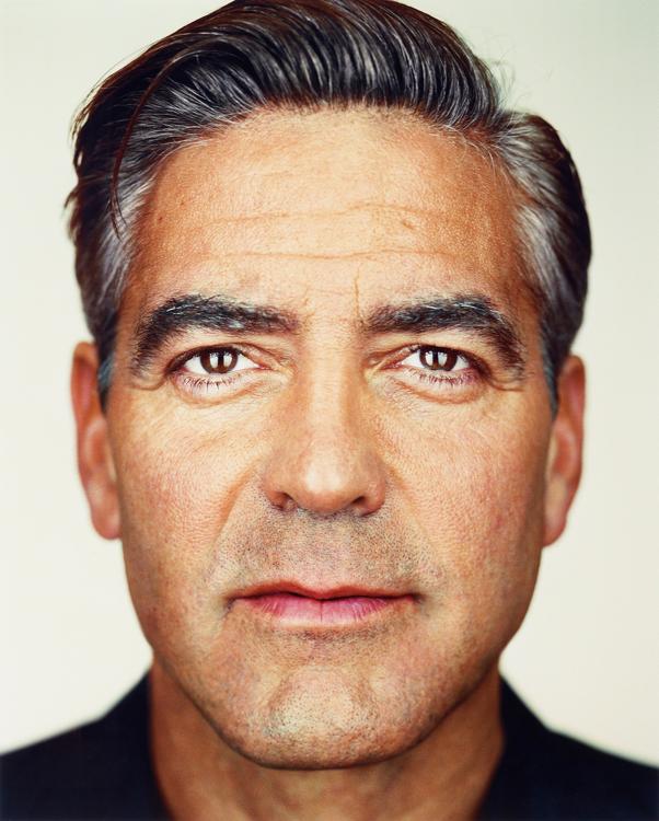
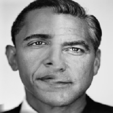
We then got to create hybrid images! These are when two images are combined and interpreted differently at different distances when looking at them. It happens by combining the higher frequencies from one image to the lower frequencies from the other. Then, at closer distances, you can see the higher frequencies while at further distances, you can see the lower frequencies. I have my images below.
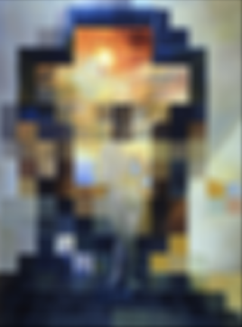
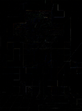
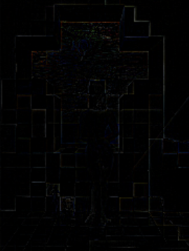
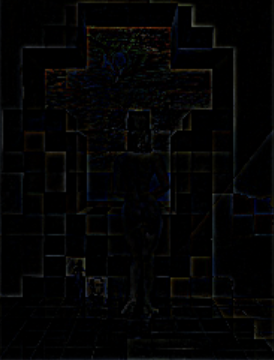
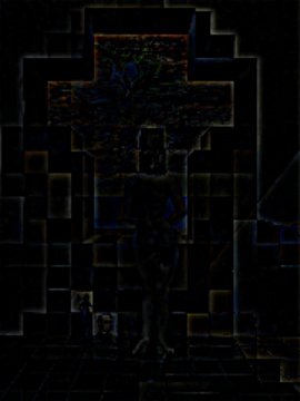
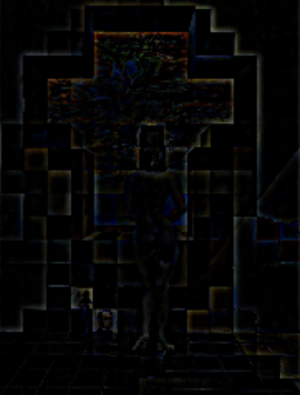
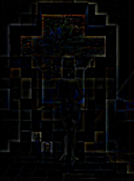
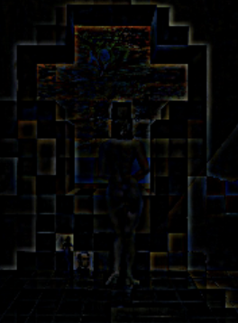
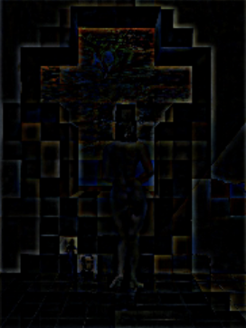
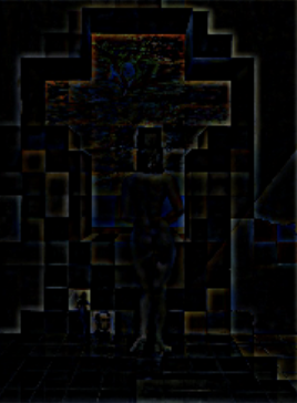
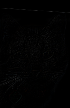
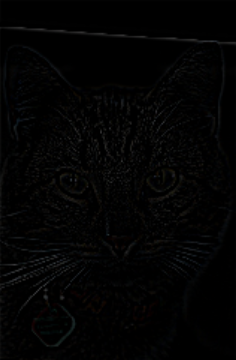
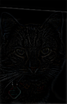
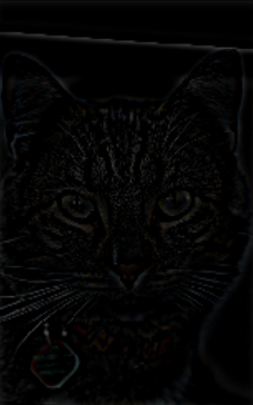
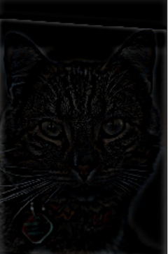
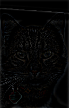
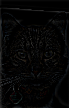
By taking the Gaussian and Laplacian stacks, we can see the image at different resolutions. I repeatedly blur an image with a kernal of size 30 and a sigma of size 6. The deeper you go in the gaussian stack, the more clear the original low frequency image becomes. The deeper you go in the laplacian stack, the higher frequency images become clearer. You will see however that my laplacian images, even though the right process is happening, are very dark. This is a clipping issue that me and a TA were having trouble figuring out. But regardless of that, you can still makeout that the further you go in the laplacian stack, the higher frequencies are becomming clearer.


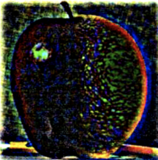
Multiresolution blending happens by blending two images using laplacian and gaussian stacks to create a smooth transition with a mask. Below are the results that I got on the orange apple and my own results (including the failed image).

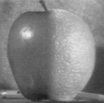

The Bells and Whistles I did were colored images for 2.2 Hybrid images (see above). Also, for 2.3 I attempted to do colored multiresolution and it came out kinda colored but my bug is that the image is quite dark and I believe it has something to do with clipping. But regardless you can kinda see how the apple is blended with the orange. (see below)
I thought this project was super cool because the baselines for the filters we see on Snapchat and Instagram are all based on the concepts we are learning from this project. I think one of my favorite things to learn about were the Gaussian filters because we used then in every single part of this project and it was amazing to see how important they are in creating that final image. The other thing I thought was really cool was the concept of low frequency being seen at further distances vs high frequency being seen at closer distances and I thought this was awesome to see applied in CS because I have seen it in my Perception psychology class. This project is awesome!