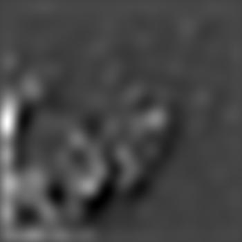
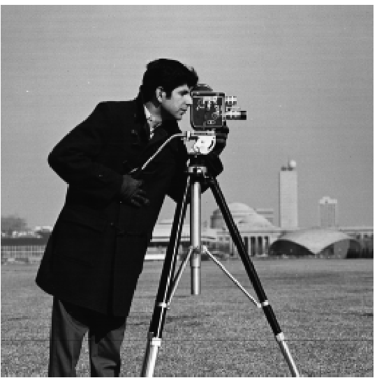
This part involves performing edge detection on this picture of a camera man.
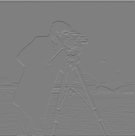
The gradient magnitude of the image is computed as follows: first compute the partial derivative in x of the image by convolving it with [[1, -1]], then the partial derivative in y by convolving with [[1],[-1]]. Then compute the gradient magnitude = sqrt(dx^2 + dy^2).
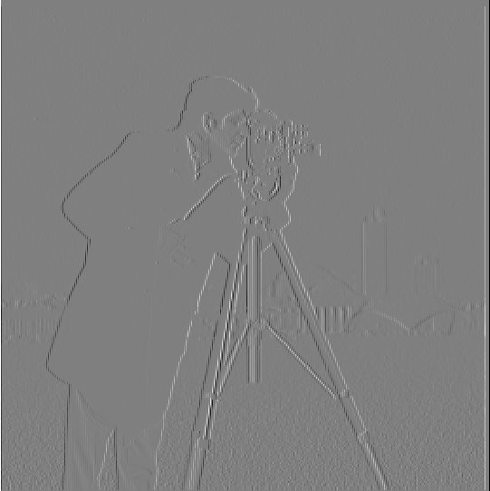
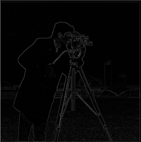
We can also binarize the gradient magnitude image using an experimentally chosen threshold to try to reduce the noise and while keeping the edges. Here the edge image is binarized with a threshold of 0.2.

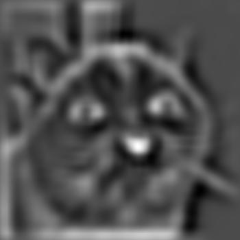
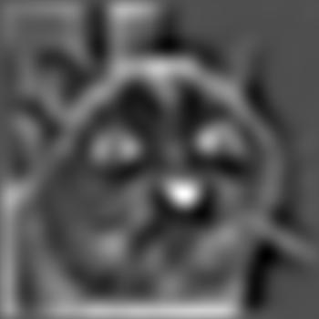
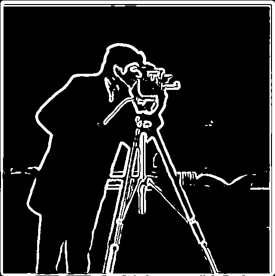
In this part we explore the effect that blurring has on edge detection for an image, and show the commutative property of convolution by showing that the binarized magnitude image produced by blurring using a Gaussian then taking the derivative is the same as the one produced by convolving an image with a DoG (convolution of a gaussian and D_x/D_y). DoG's can be reused for many images and only need to be computed once!
The main difference here is that the lines are a lot thicker and there is less noise. This is becuase the gaussian filter blurred the photo and made some of the surrounding pixels take on values that are similar to the actual edge pixels. Similarly, noise is smoothed out since those pixels take on values closer to non-edge pixels.
The gaussian filter is 9x9 with sigma = 2 for the following. The binarization threshold is 0.05.

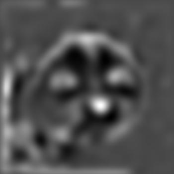
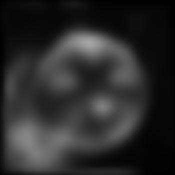
As expected, the results are the same. Below are the DoGs visualized.


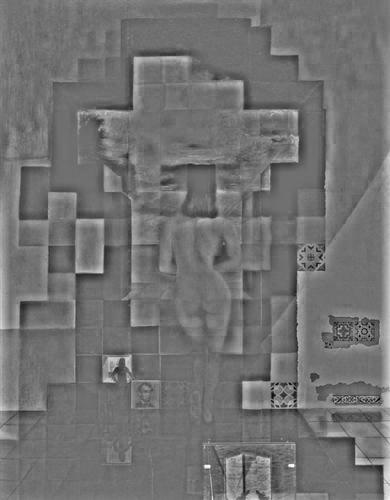
In this part we create an image straightener that works by rotating an image such that the number of vertical and horizontal edges are maximized.
I tried angles from -20 to 20 in increments of 2, G(9, 2).
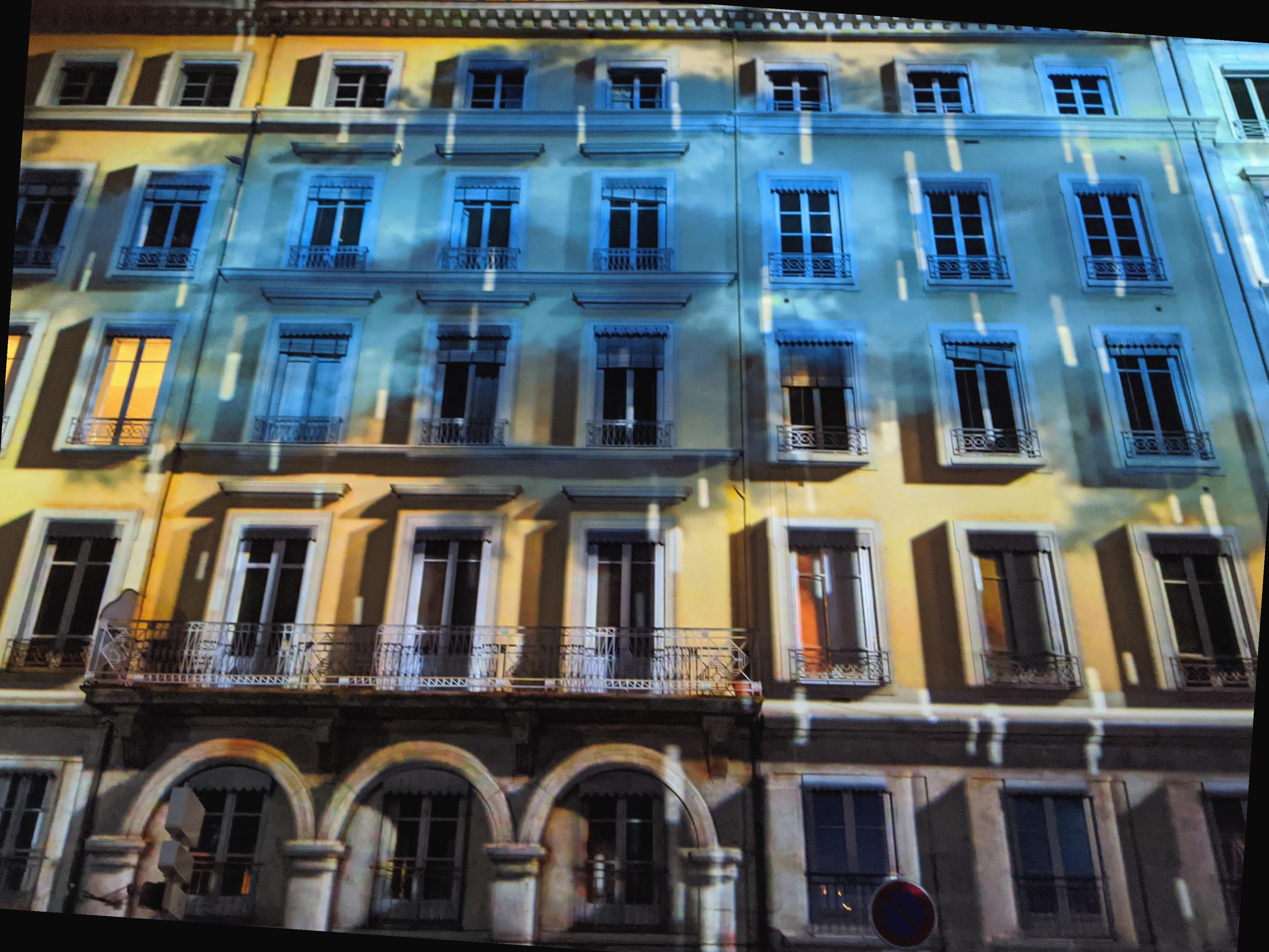
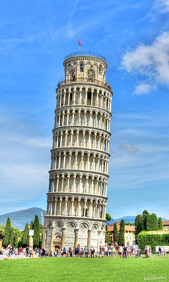
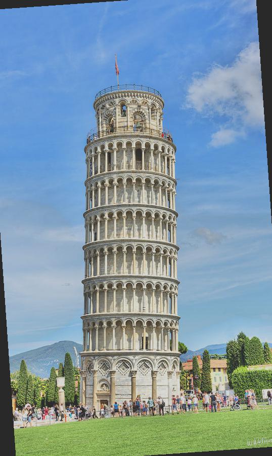
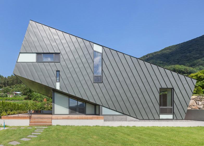
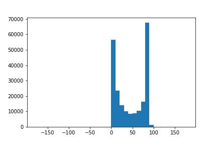

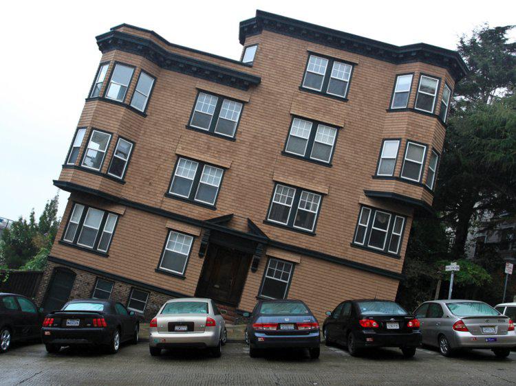
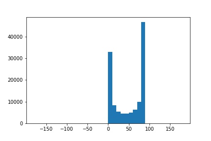
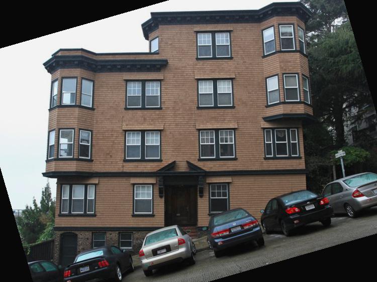
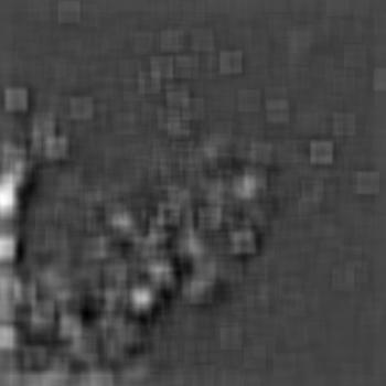
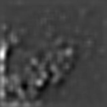
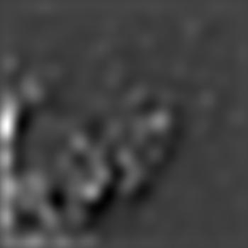
This last case failed to straighten the tilted house. Interestingly, the final rotation angle computed was 0. This may be due to the other straight lines/edges in the picture such as the pattern on the house and the windows that are not parallel or perpendicular to the outline/shape of the house itself.
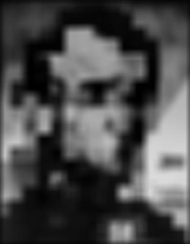
In this part we "sharpen" an image by adding the high frequencies to the image, essentially making it look sharper without using any additional information. The high frequencies are obtained by subtracting the low frequencies (blurred image) from the original image.

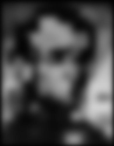
Here we blur an image before sharpening just for comparison. The final sharpened image is sharper than the blurred version, but still less sharp than the original.

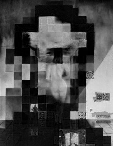
We can create hybrid images that look like one image up close and another from far away. This is done by first aligning the images, then taking the high frequencies from one image and overlaying it on top of the low frequencies of another image using methods discussed in previous parts. The high frequency image is seen up close while the low frequency image is seen from far away.


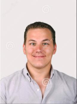

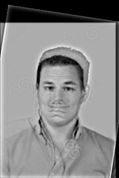


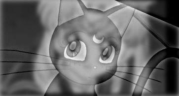
The hybrid above is a failure case since usagi and luna don't have similar face shapes and it's quite obvious usagi is overlaying way past the borders of luna's face. Although if your eyesight is as bad as mine, it's quite possible that only usagi is still visible from far away :')
Here we create Gaussian and Laplacian stacks, which are like the pyramids except with no downsampling \o/ The Gaussian layers are made by repeatedly blurring the original image, and the Laplacian layers are made by taking the difference between the successive Gaussian layers.


We can also blend two images A and B together seamlessly with mask M using the stacks described in 2.3! The computation is as follows: build laplacian stacks LA and LB for images A and B respectively, build a gaussian stack GM for the mask M, form a pyramid LS where for each level i LS(i) = LA(i)*GM(i) + LB(i)*(1 - GM(i)), then obtain the final splined image by summing the levels of LS.
Note that we must add an extra layer to the laplacian stacks that is the same as the last level of the corresponding gaussian stack so that you can get back the original image through summing.
I first tested using the apple/orange example given, then generated the new splines below.