This project experiments with various filters and 2D convolutions in the exploration of a variety of image processing techniques.
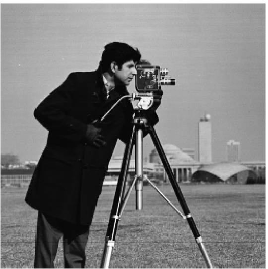
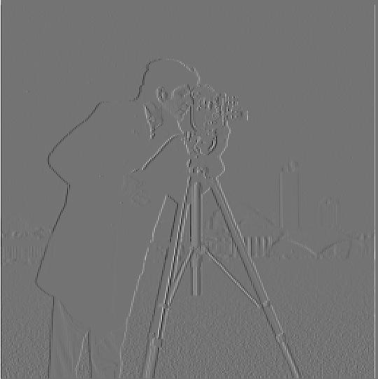
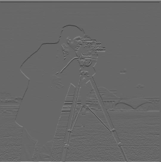
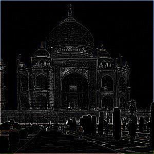
In this part I use finite difference operators for edge detection. By convolving an image with the simple kernels [1, -1] and [1, -1].T, the resulting images represent the image's horizontal and vertical gradients, respectively.
| Original | Horizontal Gradients (convolved with D_x) | Vertical Gradients (convolved with D_y) |
|
|
|
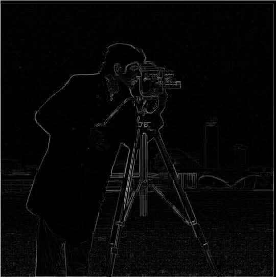
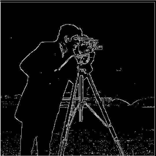
We can combine the above results to find the gradient magnitudes at each pixel. Specifically, for each pixel, we just take the norm of the gradient vector ||[dx, dy]|| = sqrt(dx^2 + dy^2). With the resulting gradient magnitude image, we can set some arbitrary threshold for the gradient magnitudes to filter out most of the noise and get only the relevant edges:
| Gradient Magnitudes | Thresholded Magnitudes (Threshold Value = 0.18) |
 |
 |
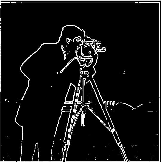
There's still a bit of noise in the result above, so I apply a gaussian kernel (size = 3, sigma = 1) to smooth the image before applying the same process as before. The edges have much less noise in the resulting image.
| Without Gaussian Kernel | With Gaussian Kernel |
|
 |
Applying the gaussian kernel to the image adds a convolution to the process, but luckily, as convolutions are associative, we can optimize this a bit by applying the finite difference kernels to the gaussian kernel. Here are the resulting kernels:
| Derivative of Gaussian Kernel on X | Derivative of Gaussian Kernel on Y |
 |
 |
Using these kernels results in the same final image, with one fewer convolution!
| Pre-applying Gaussian Kernel | Using Derivative of Gaussians |
|
 |
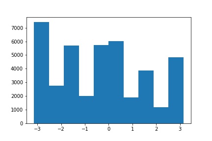
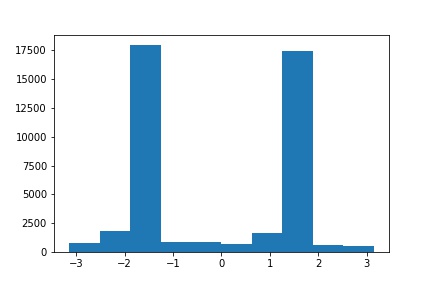
Using our edge detector, we can create a image straightener that searches for possible image rotation angles and picks the one with the straightest edges. Specifically, we can get the gradient angle at a given pixel using the derivative results (using the Derivative of Gaussian Kernels from the previous part) at the pixel: theta = arctan(dy / dx). For this part, my Derivate of Gaussian kernels used a gaussian kernel with size = 5 and sigma = 2.
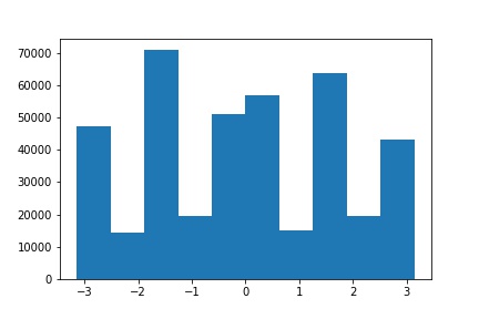
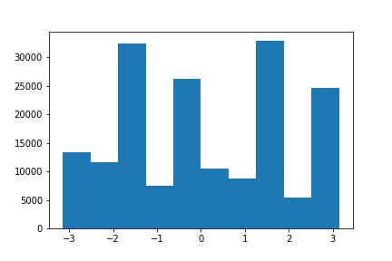
Using the same edge detection process as in part 1.2, I devised a simple metric for how "straight" the overall image was. For all the edge pixels, I compute the gradient angles and return the mean of squared differences to the closest of: -pi, -pi/2, 0, pi/2, or pi (as these are axis-aligned). Since straighter edges will have more gradient angles close to one of those axis-aligned values, straighter images will have a smaller mean squared distance.
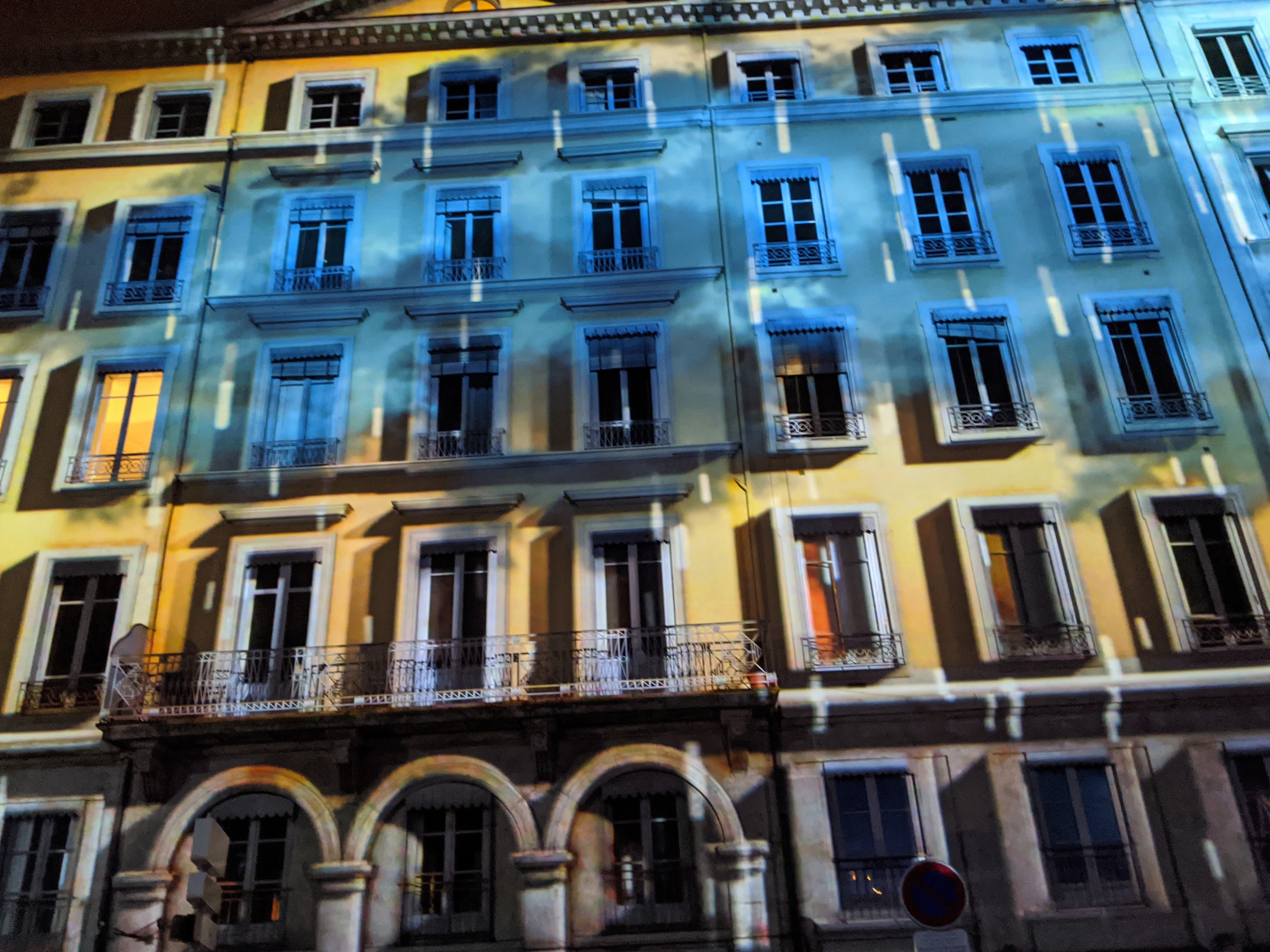
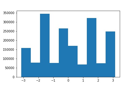
Finally, since rotating the image will create edges along the rotated border of the image, I only compute this metric for the center square of the image, whose side length is 1/2 the horizontal side length of the original image. Below are the results of this process on a few images, along with a histogram of angles for each image.
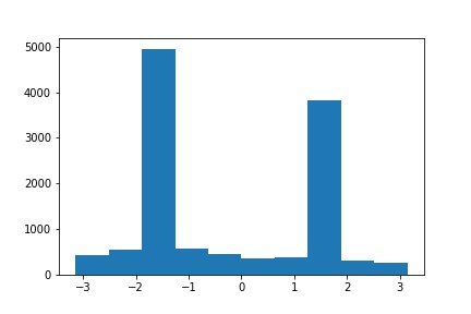
| Original | Original Orientation Histogram |
 |
 |
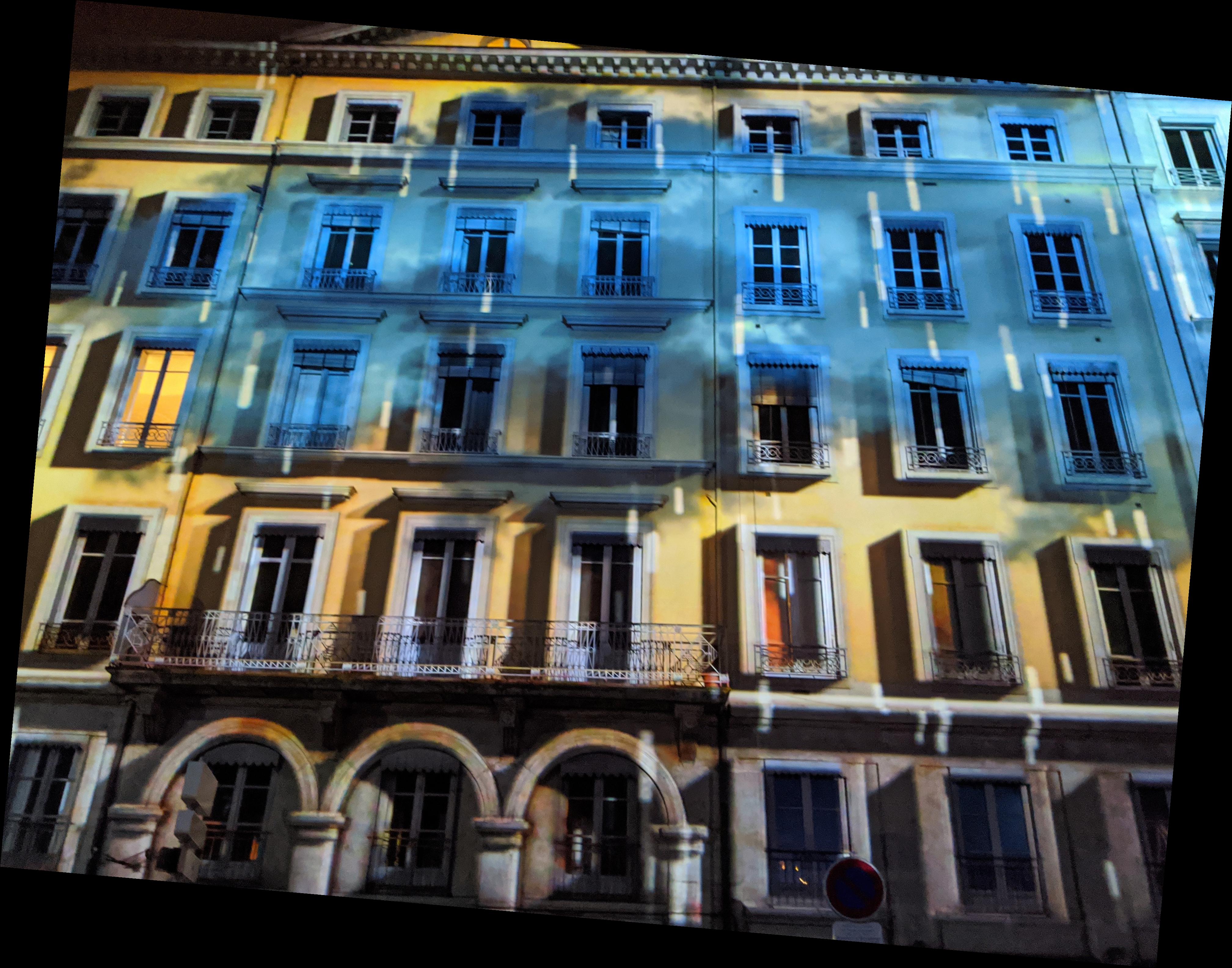
| Straightened (Angle = -5) | Straightened Orientation Histogram |
 |
 |
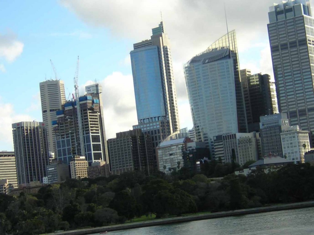
| Original | Original Orientation Histogram |
 |
 |
| Straightened (Angle = -8) | Straightened Orientation Histogram |
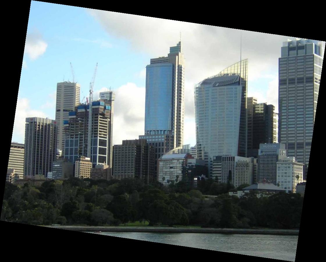 |
 |
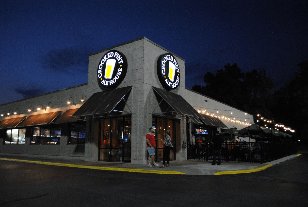
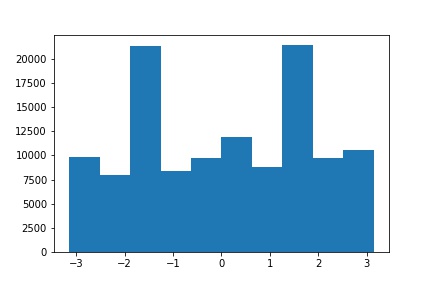
| Original | Original Orientation Histogram |
 |
 |
| Straightened (Angle = -7) | Straightened Orientation Histogram |
 |
 |
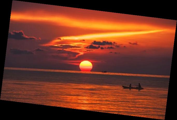
| Original | Original Orientation Histogram |
 |
 |
| Straightened (Angle = 9) | Straightened Orientation Histogram |
 |
 |
This approach performed the best on the Facade and Skyline images. For Horizon, the image is still not perfectly straight. This is likely due to the streaks of clouds in the sky, which are detected as edges. Since these edges are not parallel to the horizon, the metric picks an angle that is somewhat in-between straightening either just the clouds or just the horizon. To mitigate this issue, it may be worth considering changing the metric to counting the number of edge angles within a certain threshold from one of the axis-aligned values, instead of taking the sum of squared distances. For Onalaska, the picture was originally straight. However, since the picture is taken at the corner of a building, the algorithm attempts to align the image to one of the diagonal edges along the building's roof, causing it to skew the image significantly.
We can artificially "sharpen" an image by adding accentuating the high-frequency components. The process is as follows:
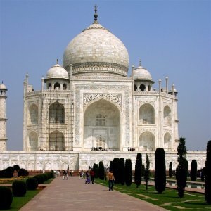
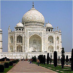
For Taj, I used alpha = 4 and a gaussian of size = 3, sigma = 1.
| Original | Blurred | Alpha * High Frequencies | Sharpened |
 |
 |
 |
 |
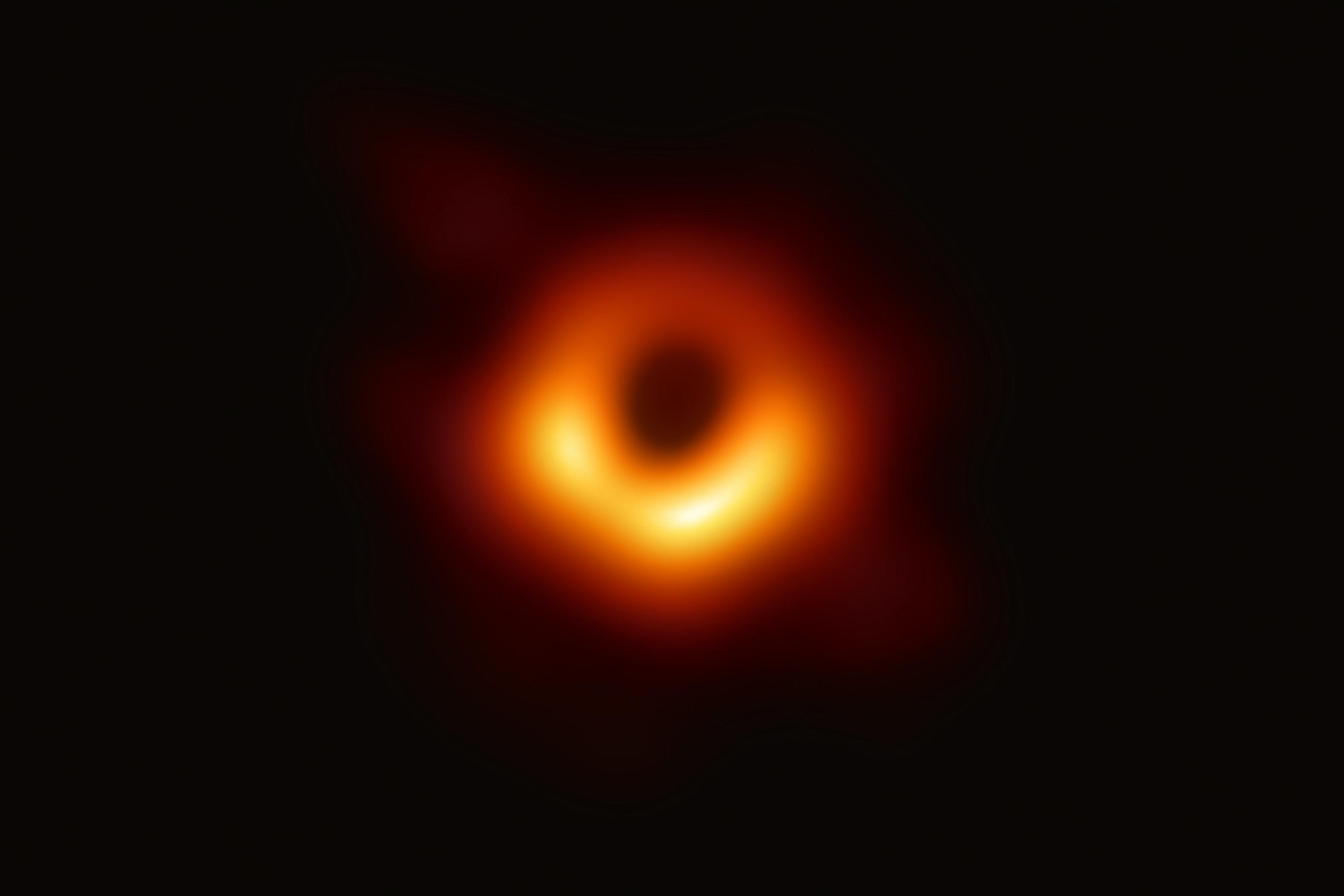
For Black Hole, as the original image was very blurry, I used a larger alpha = 300 just to make the differences between the original and final image more visible.
| Original | Blurred | Alpha * High Frequencies | Sharpened |
 |
 |
 |
 |
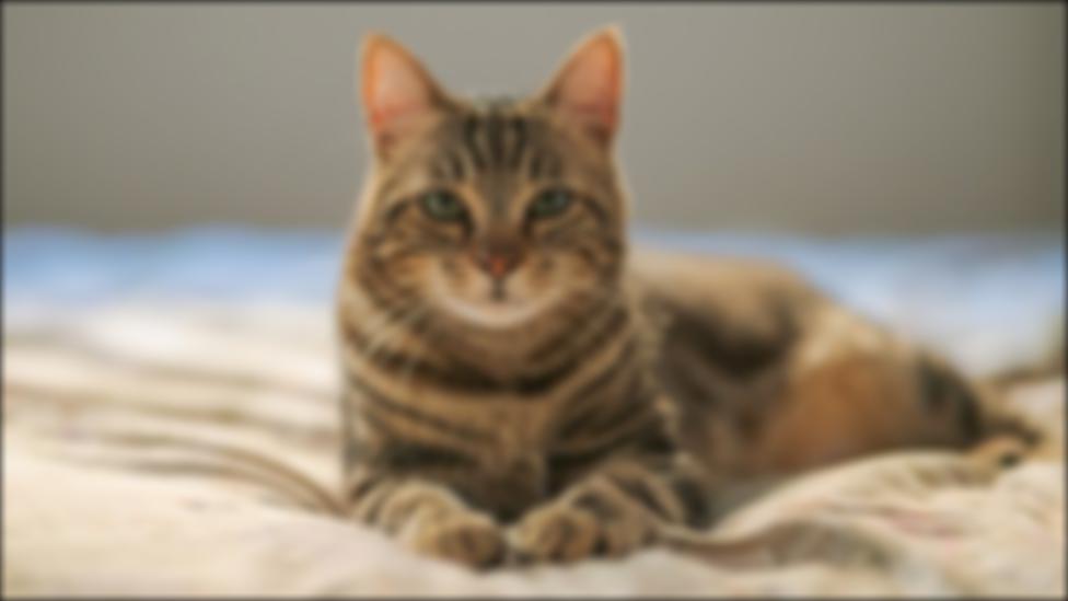
Obviously, as the original image contained very little high frequencies to begin with, the black hole image did not sharpen well. To expand upon this, I took a sharp image (Cat), blurred it, then attempted to sharpen the blurred result. Because the unsharpen mask only accentuates existing high frequency signals, the final result doesn't look as good as the original, sharp image.
For Cat, I blurred the image with a gaussian kernel of size = 15 and sigma = 5, then sharpened the image with alpha = 70.
| Original | Blurred | Sharpened |
 |
 |
 |
This part creates Hyrbid Images by blending the high-frequency portion of one image with the low-frequency portion of another, such that at different distances different images are percieved. For my high- and low-pass filters, I use gaussians with size = 12 and some specified sigmas. For the high-pass, the kernel is the gaussian subtracted from the unit impulse. From looking at the results from the color images below, it seems like color works best for the low-frequency component of the image.
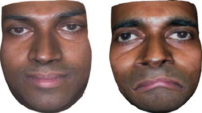
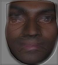
For this image, I low-passed (sigma = 4) the smiling face and high-passed (sigma = 2) the frowning face. Up close, the face looks like it is frowning, while from afar, it looks like it is smiling.
| Original Images | Hybrid Image |
 |
 |
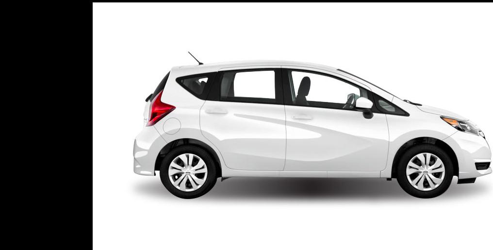
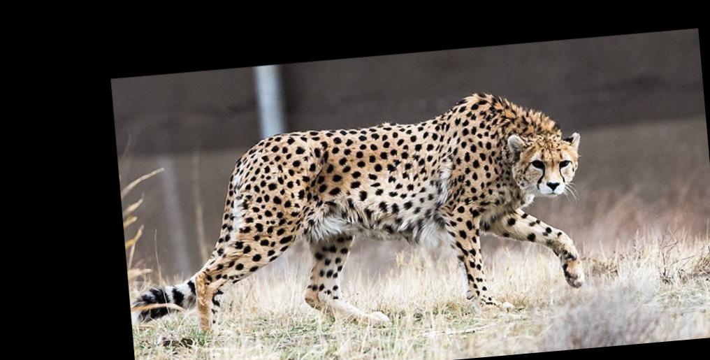
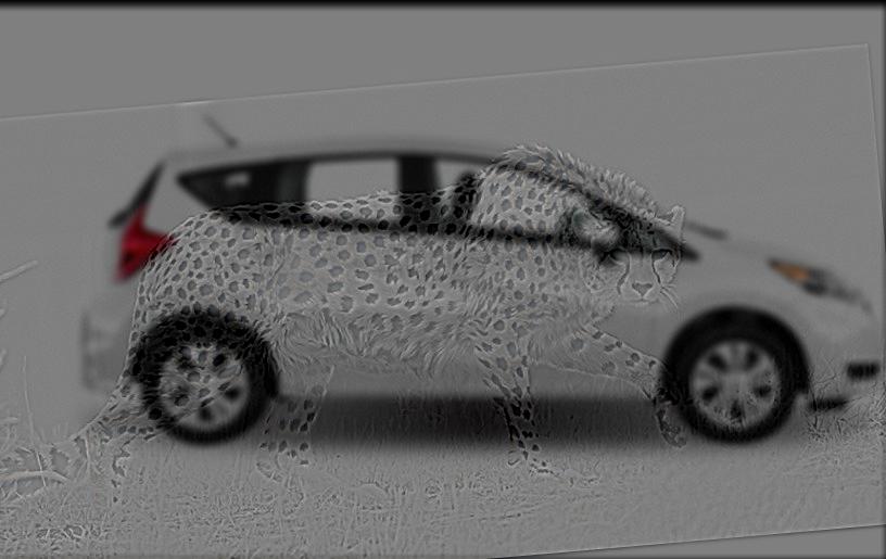
I low-passed (sigma = 4) the car and high-passed (sigma = 2) the cheetah. Unfortunately, this image doesn't work very well, as even up close the car is still fairly easy to see in comparison to the cheetah. This may be because it's difficult to align the two images, as the car and cheetah are not entirely the same shape, and the car has some vibrant colors (red taillight) that stand out.
| Car | Cheetah | Hybrid Image |
 |
 |
 |
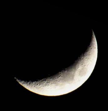
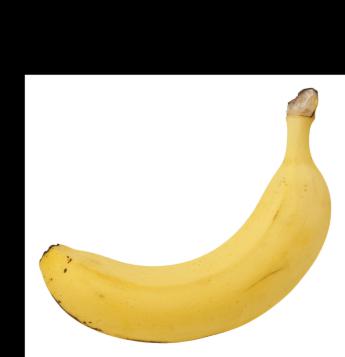
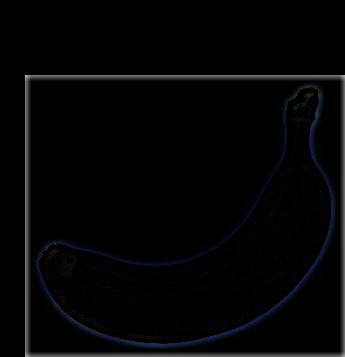
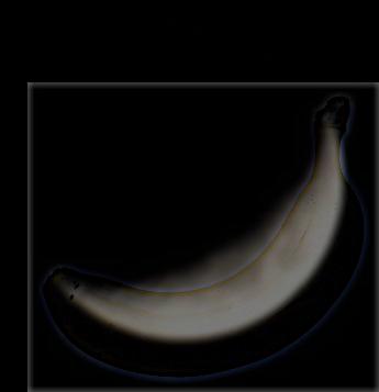
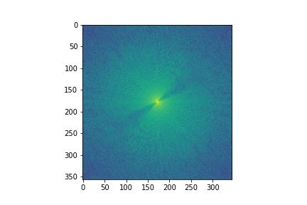
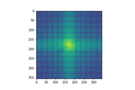
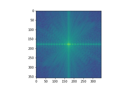
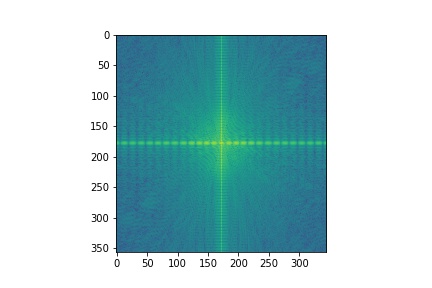
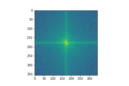
I low passed (sigma = 4) the moon and high-passed (sigma = 8) the banana. I've also included the log magnitude of the fourier transform of the images and intermediate results. As expected, the filtered moon image is primarily composed of low-frequencies, while the filtered banana has more high-frequencies.
| Moon | Filtered Moon | Banana | Filtered Banana | Hybrid Image |
 |
 |
 |
 |
 |
 |
 |
 |
 |
 |
I implemented a Gaussian stack, where at each level the previous level's image is convolved with a gaussian filter. To construct a Laplacian stack for the image, for the i-th level of the stack, I subtract the i+1-st level of the gaussian stack from the i-th level of the gaussian stack.
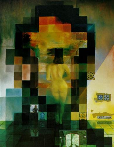
Below I construct a Gaussian and Laplacian stack for Dali's Lincoln painting. Each stack has a 5 levels, and each level is convolved with a gaussian filter with size = 6 and sigma = 2.
| Original | Gaussian Stack |
 |
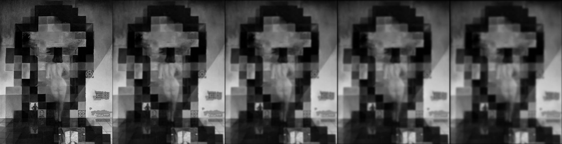 |
| Laplacian Stack | |
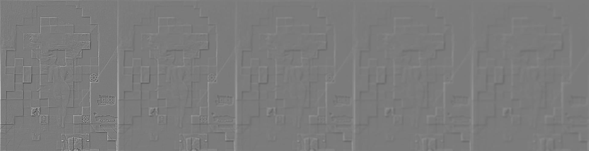 |
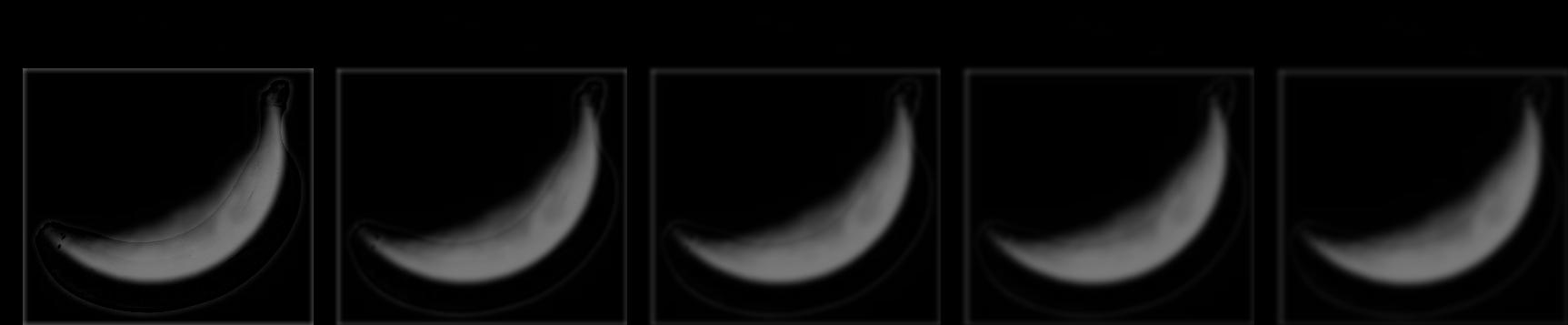
Below I also construct a Gaussian and Laplacian stack for the Banana / Moon hybrid image from Part 2.2. Each stack has a 5 levels, and each level is convolved with a gaussian filter with size = 6 and sigma = 2. As expected, the first few levels of the Laplacian stack, which contain the higher frequencies of the image, have a more clearly visible banana, but in the lower levels, only the moon is visible.
| Original | Gaussian Stack |
|
 |
| Laplacian Stack | |
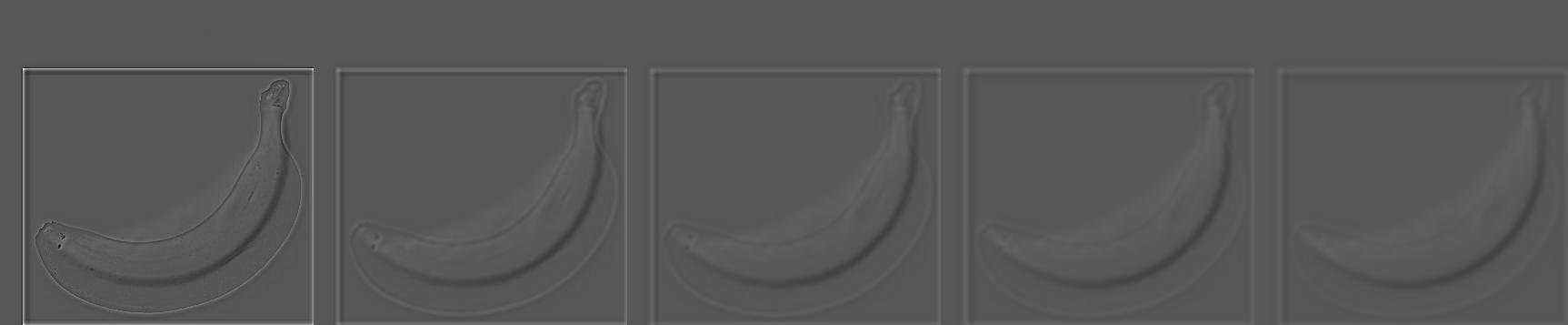 |
Blending images together requires two images and a mask. We first generate Laplacian stacks (LA and LB) for the two images, and a Gaussian stack (GR) of the mask. Then at each layer, we generate a new laplacian stack that is convex combination of LA and LB, weighted by GR. Summing up the layers of this new stack (along with the final gaussian layers) yields the blended result. Below I have a few examples from this process.
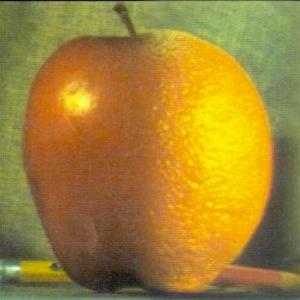
I blended the two images with a simple vertical split as the mask. The Gaussian and Laplacian stacks had a depth of 5 and used a gaussian with size = 30 and sigma = 10.
| Apple | Orange | Mask | Blended Result |
 |
 |
 |
 |
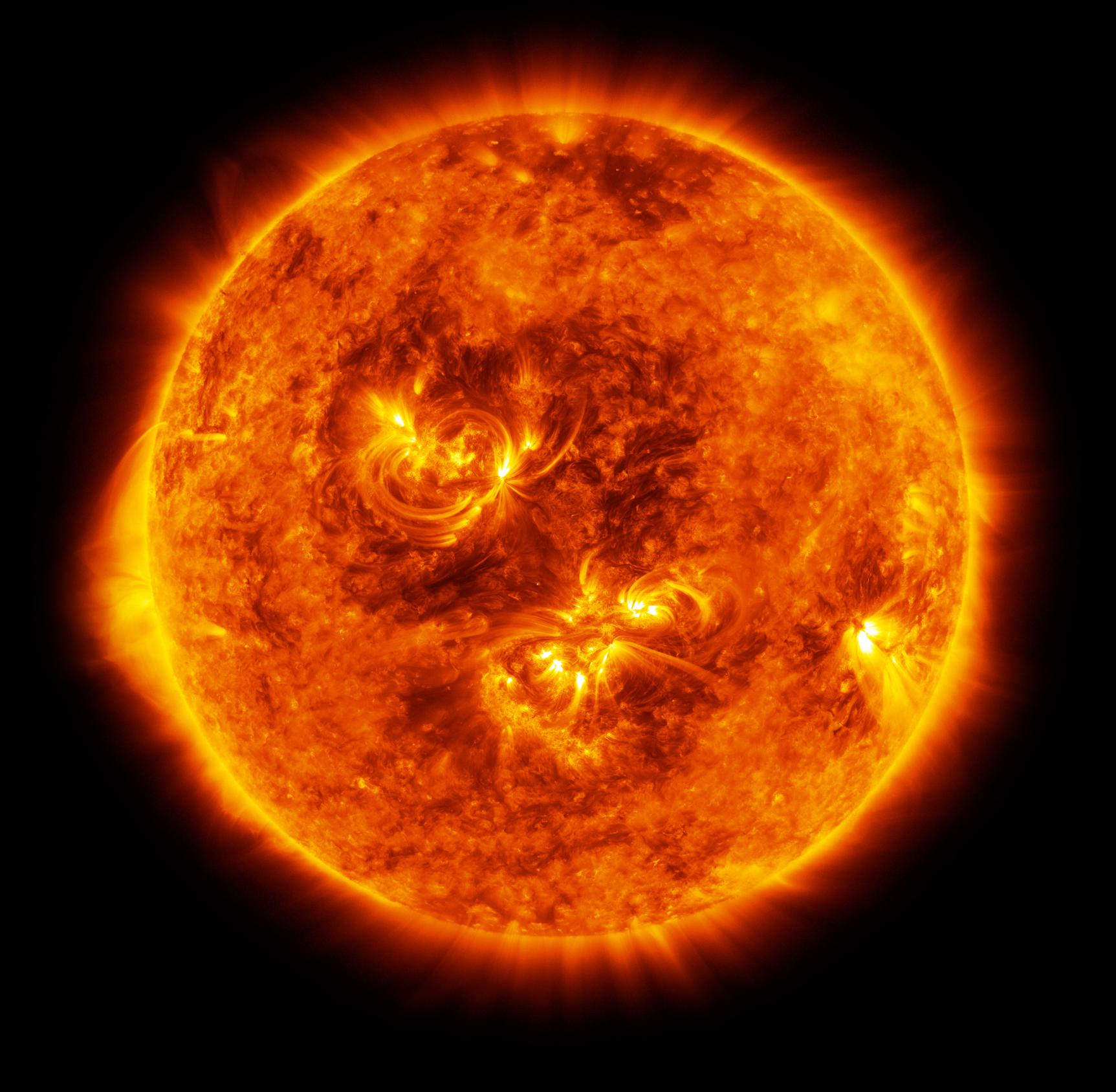
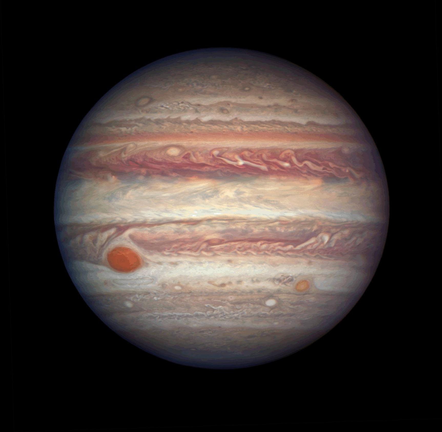
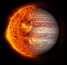
Similarly, I blended images of the Sun and of Jupiter using the same vertical mask. The stacks had a depth of 5 and used a gaussian with size = 30 and sigma = 30.
| Sun | Jupiter | Mask | Blended Result |
 |
 |
 |
 |
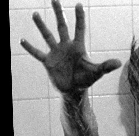
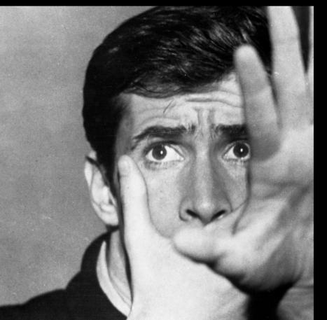
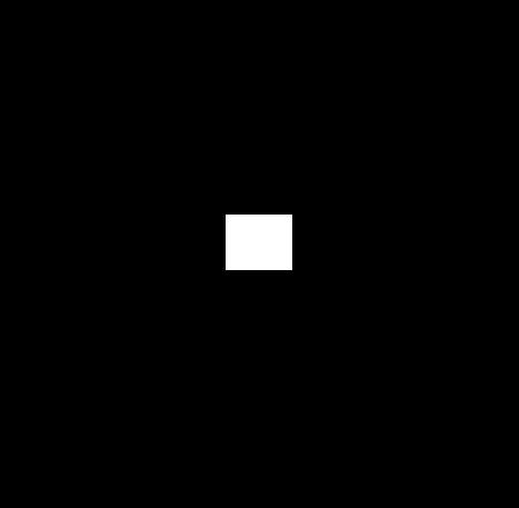
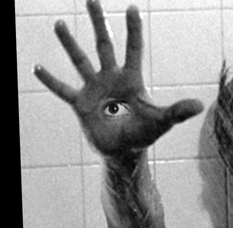
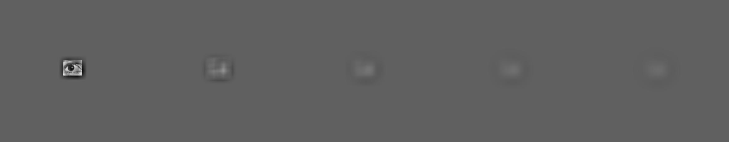
I used images from Psycho to generate an image of an eye in a hand. Here, the mask is a square near the center of the image (surrounding the eye). The stacks had a depth of 5 and used a gaussian with size = 30 and sigma = 30.
| Hand | Eye | Mask | Blended Result |
 |
 |
 |
 |
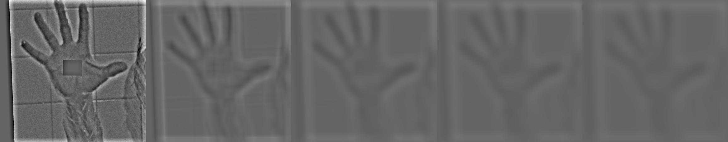
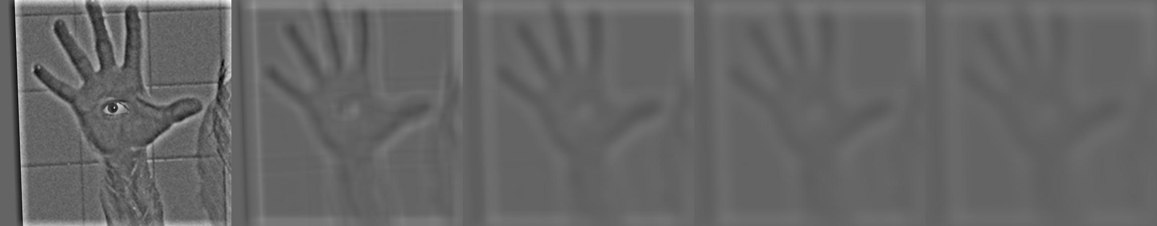
Below are the Laplacian stacks for each of the masked input images and of the blended result.
| Hand Laplacian Stack |
 |
| Eye Laplacian Stack |
 |
| Blended Laplacian Stack |
 |