In this project the goal is to familiarize ourselves with filters and frequencies and understand their roles in image manipulation. By experimenting with gaussian blurs, derivative filters, and laplacians, it was easy to understand the strength of simple filters on image manipulation.
For the first part of this project, different aspects of filtering were explored. Using derivative filters, gaussian blurs, and algorithms to estimate the best rotation to straighten an image or for edge detection, I was able to create a wide range of outputs that are included below.
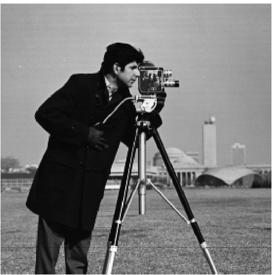
1.1: Finite difference operator.
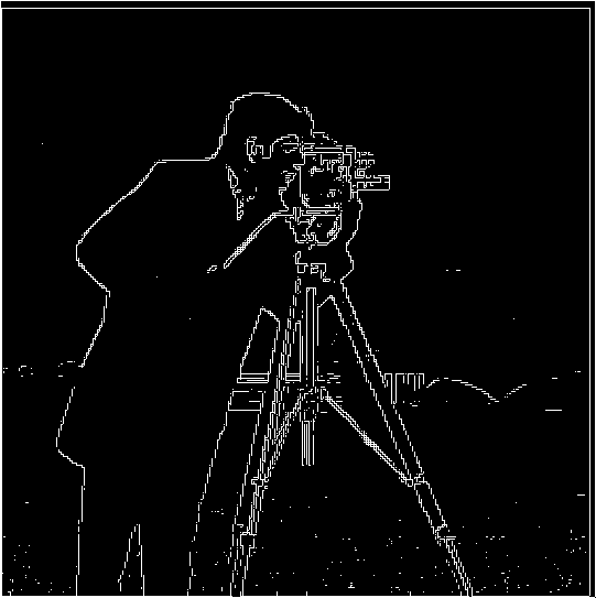
By taking the finite difference operators Dx = [1, -1] and Dy = [1, -1]^t (transpose) I was able to create an edge detection algorithm that displayed prominent edges in pictures and filtered out some of the noise. Convolving the image in 2d with the finite difference operators Dx = [[1, -1], [0,0]] and
Dy = [[1, -1] [0, 1]] and then take its magnitude sqrt(convolve2d(image, dx)^2 + convolve2d(image, dy))^2 an image was generated of edges in the photo. The image was still noisy, so it was filtered out by only including the parts that were > 2 * std of the convolved image.
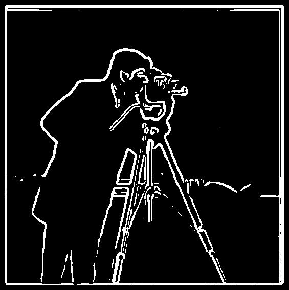
While the edge detection in 1.1 might be good, there was a way to improve it. By convolving the gaussian with the image first and then following the steps above, the image becomes a significantly higher resolution edge detection algorithm.
By convolving the image with the gaussian before applying the derivative filter, I was able to blur the image in noisier places, which made it easier to filter these places out. This meant that our output had less noise and more clear edges displayed.
Another interesting note is the ability to convolve the image with the gaussian and then the finate difference operators OR convolve the gaussian with the finite difference operator and then the image and still have the same output.

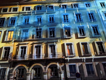
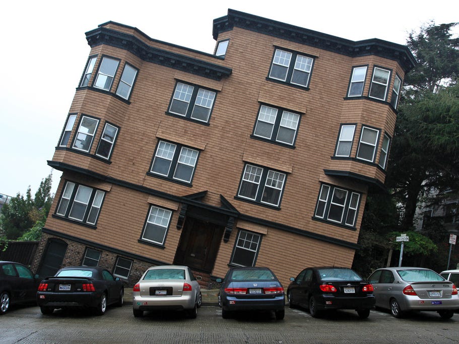
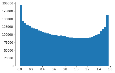
By iterating through different angles, rotating the image by these angles, convolving them with dx and dy, and then counting the angles vertical and horizontal lines using the relationship theta = arctan(dx/dy).
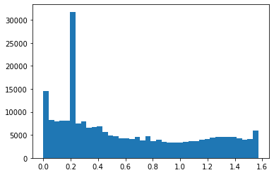
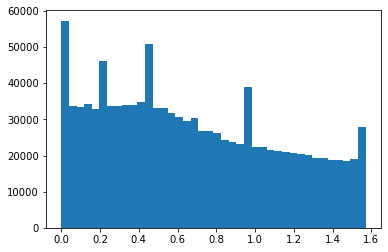
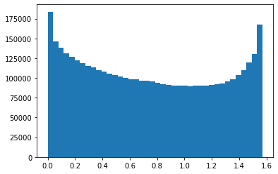
By counting the number of the theta values that represent vertical and horizontal lines, it is possible to find the best image rotation. Below are also histograms of the original and straightened images to show the distribution.
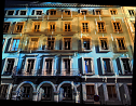
In the case of the facade image, the rotation worked well at a -3 degree rotation.


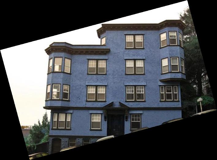
The case of the tilted San Francisco house worked well at a 1 degree rotation.
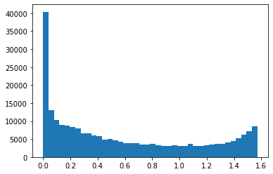
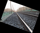
The case of the tilted train tracks worked well at a -5 degree rotation.


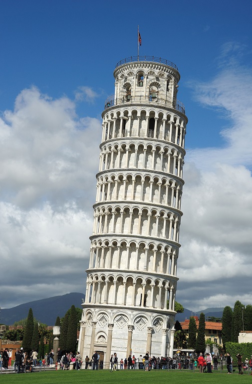
The case of the tilted building failed . The noise generated by the clouds in the background probably generated some of these issues.
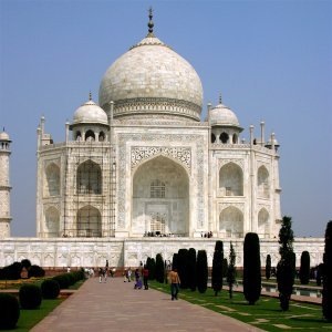
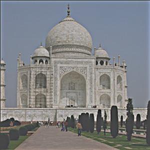
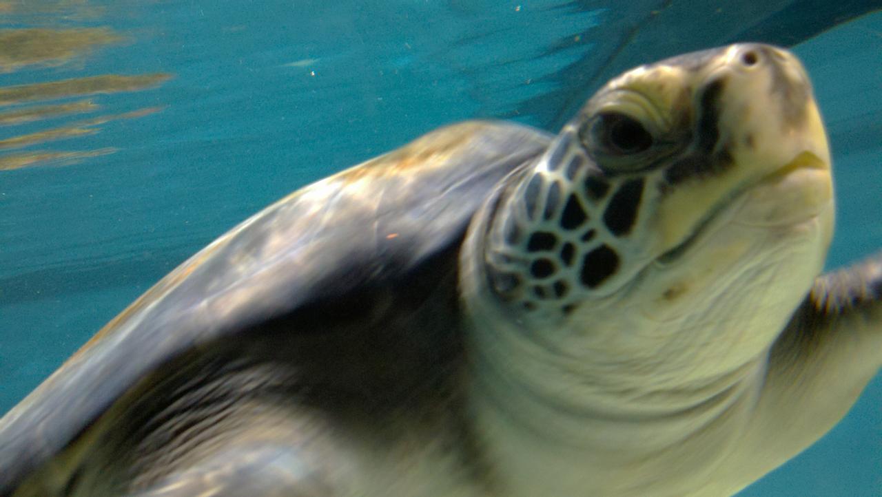
By taking an image and convolving it with the laplacian, it was possible to remove some of the noise to make it appear higher resolution.
Taj image
Sparkler image. This image appeared more blurry at the end. This could be due to how blurry the background is or the lack of strong focus on any particular part of the image
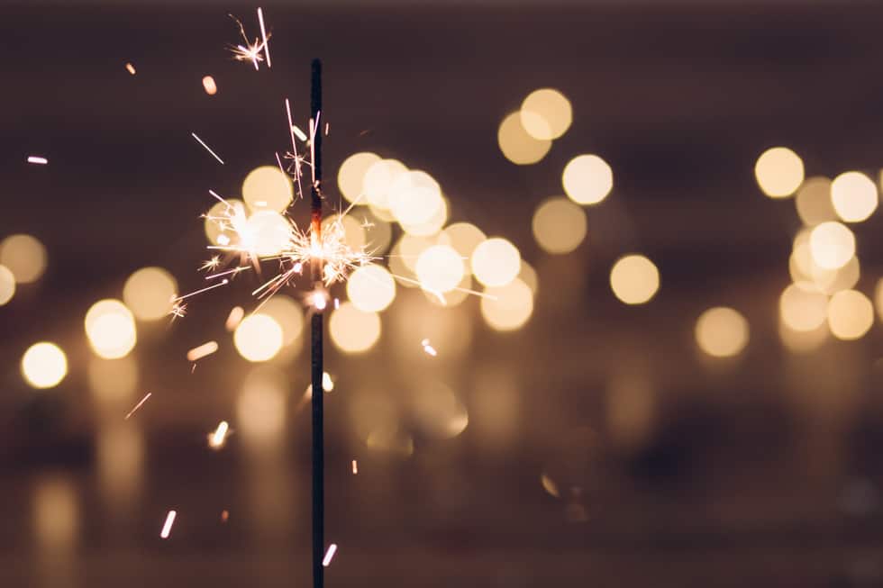
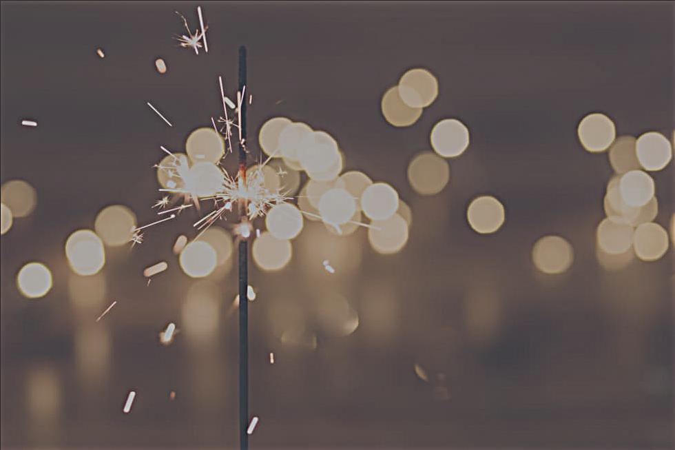
Image of a turtle
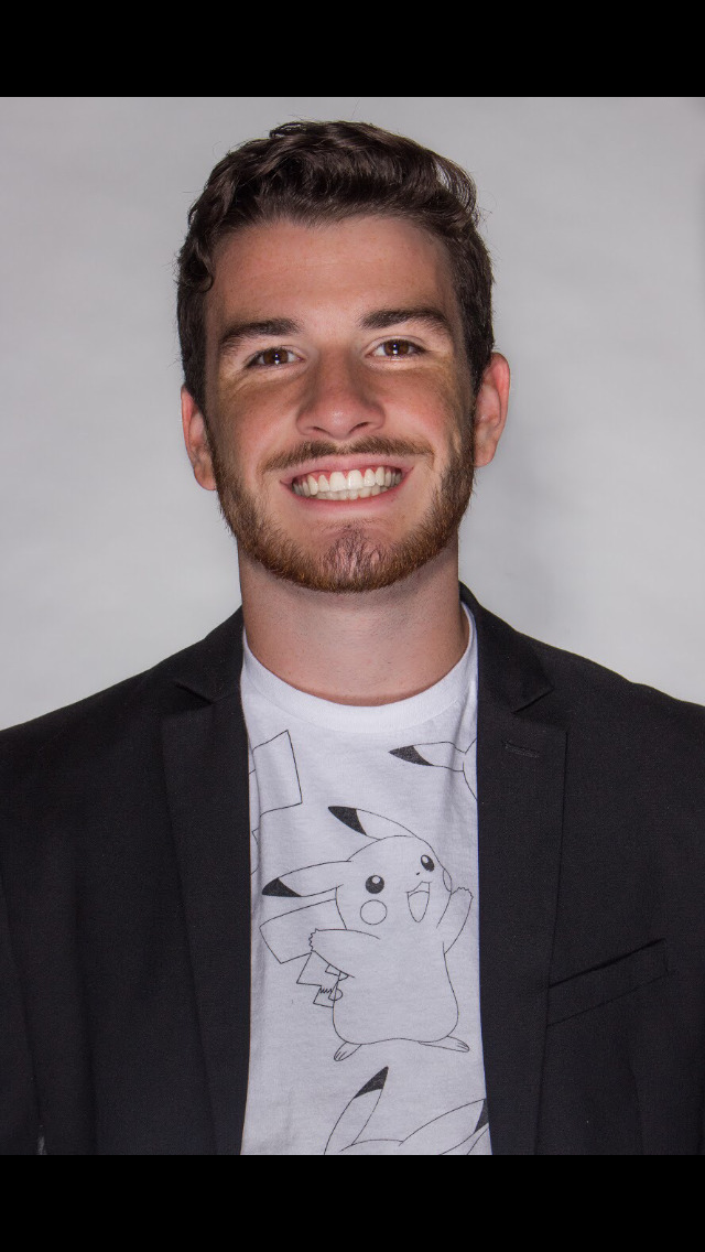
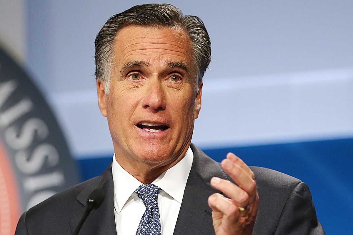
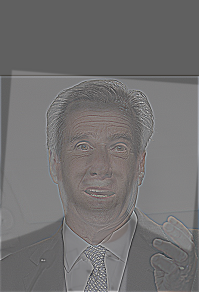
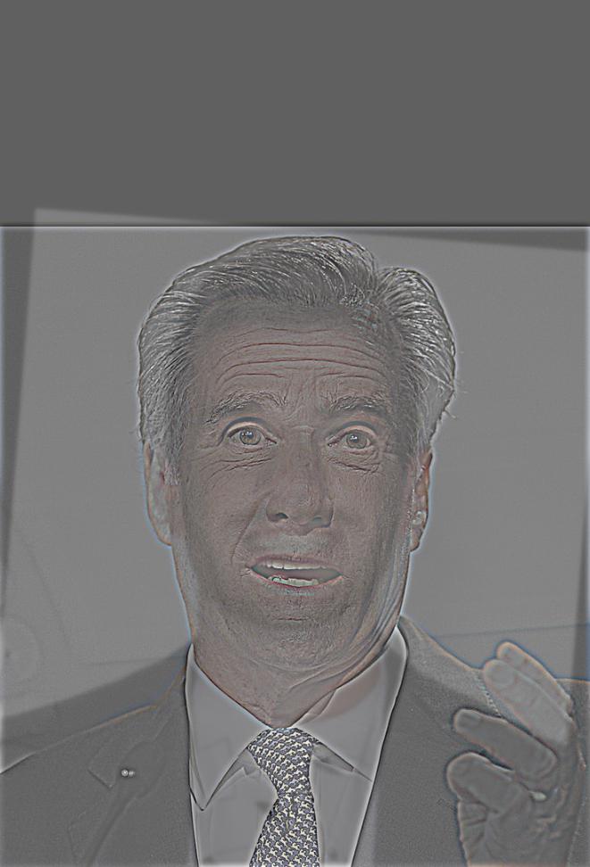
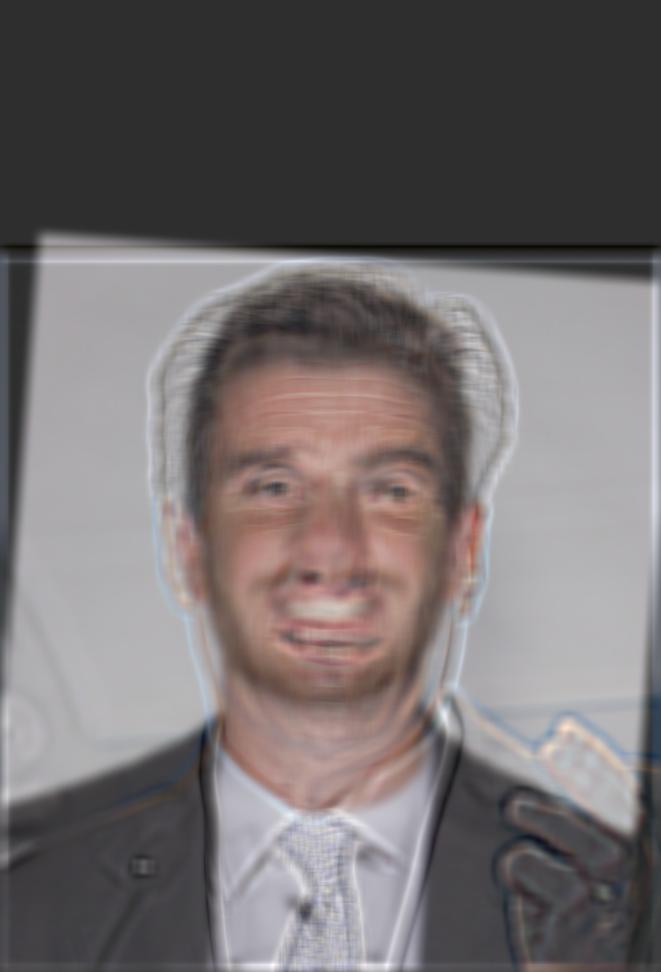
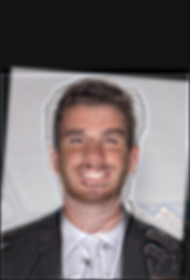
By combining images where one is filtered by a high pass filtered and the other by low pass, it is possible to create hybrid images that appear differently based on how far away you view them.
Mitt Romney + me (Romnme). I would consider this a failure due to the different shapes of our faces being very obvious. While not as conventional as a failure such as mixing two totally different objects, I thought this was a more interesting case.
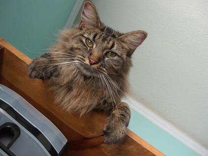
nutmeg + derekPicture

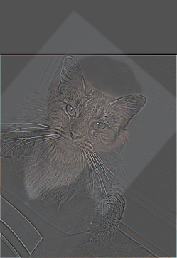
Sasuke + naruto


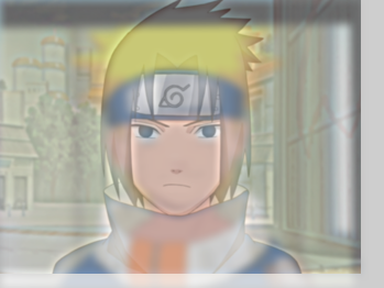
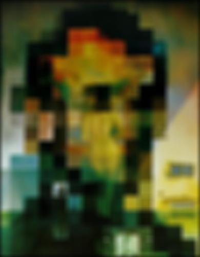
By taking images and creating gaussian and laplacian stacks, we are able to see the structure at different resolutions. Examples are shown below.
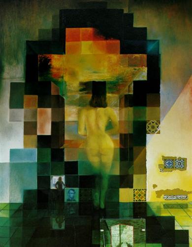
The gaussian Stacks:


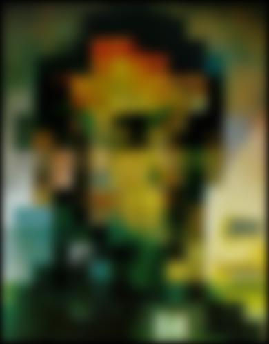
The laplacian stacks
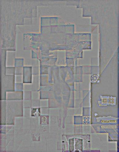
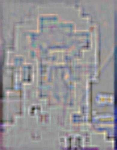
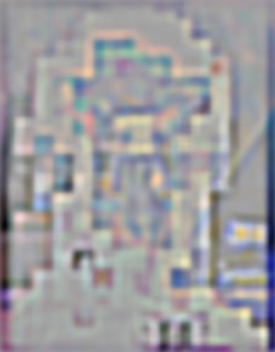

The gaussian Stacks:

The laplacian stacks


