Fun with Filters and Frequencies!
Part 1: Fun with Filters
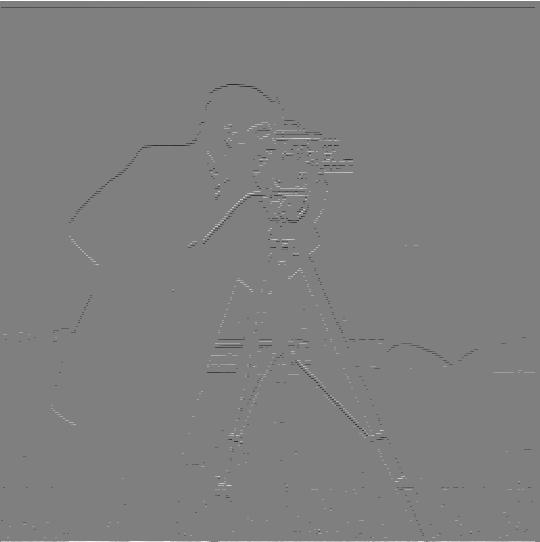
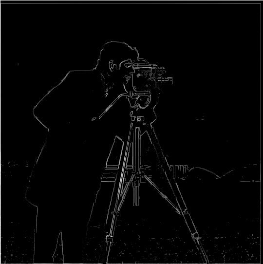
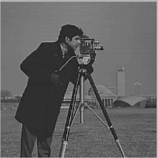
Part 1.1: Finite Difference Operator
In this part we computer the gradient of an image. What we did is we have a differene operator
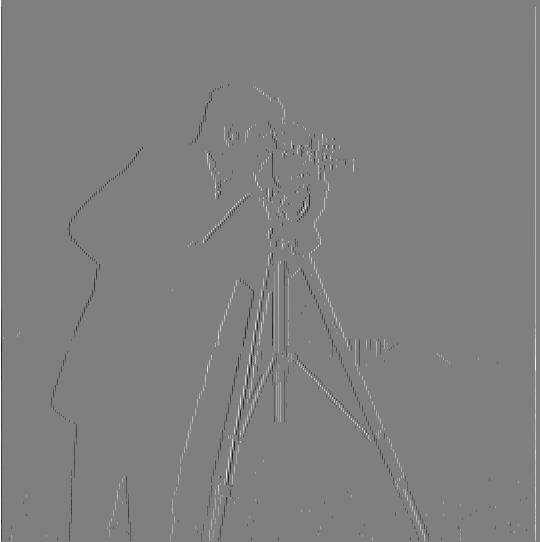
and we convolute the operator over the gray scale image, and get a x-direction derivative and y-direction derivative. Combining the two resulting in the gradient magnitude image.
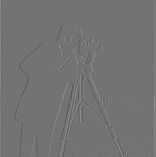
camerman x-direction derivative
camerman y-direction derivative
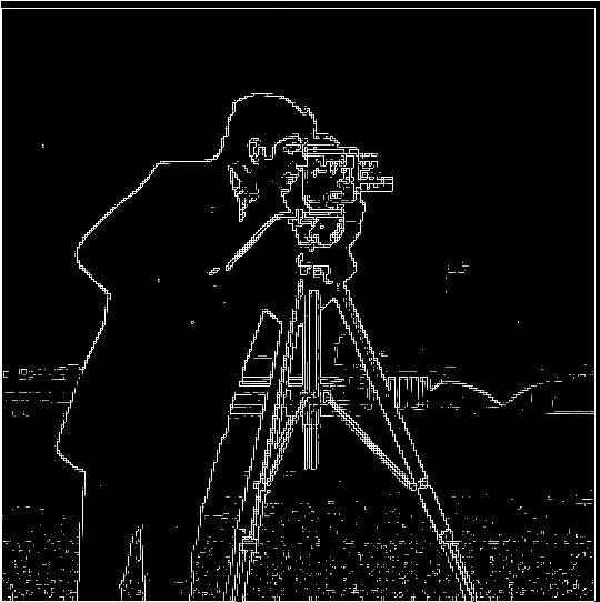
cameraman gradient image
Derivative of Gaussian (DoG) Filter
Part 1.2: Derivative of Gaussian (DoG) Filter
Now in this part, we introduce the use of Gaussian filter. We create a 2D Gaussian filter by taking the outter product of 1D Gaussian filter and its transpose. By convoluting the gray scale image and the Gaussian filter, we get a blur version of the image. Next, we computer the derivative of Gaussian on both x and y axis, and combine them into a gaussian gradient image. Notice here, we can first convolute the Gaussian filter with the difference operator, and then convolute with the image to get the same result, and it will be the so call DoG filter.
camerman image with Gaussian and dx
camerman image with Gaussian and dy
camerman image with DoG
Image Straightening
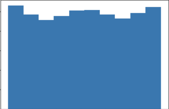
In this part, we are doing an auto-rotation for images. Notice if we use the difference operator, we can find the gradient angle by taking an arctan. The closer the absolute value of arctan to 0 or pi(90 degree) , the more "straight" it is (honrizontally and vertically). So we computer the point where we believe the image is most "straight", and rotate the image. In fact, the histogram can do the same thing. We are looking for the rotation of the image that has the most 0 or 90 degree value for absolute arctan value. I provided one failure example, which I believe the reason it fails is that our algorithmn rely on things being straight. However, in the failure case, the correct rotation angle will result in some part of the image not perpendicular to the ground, and so the result failed.
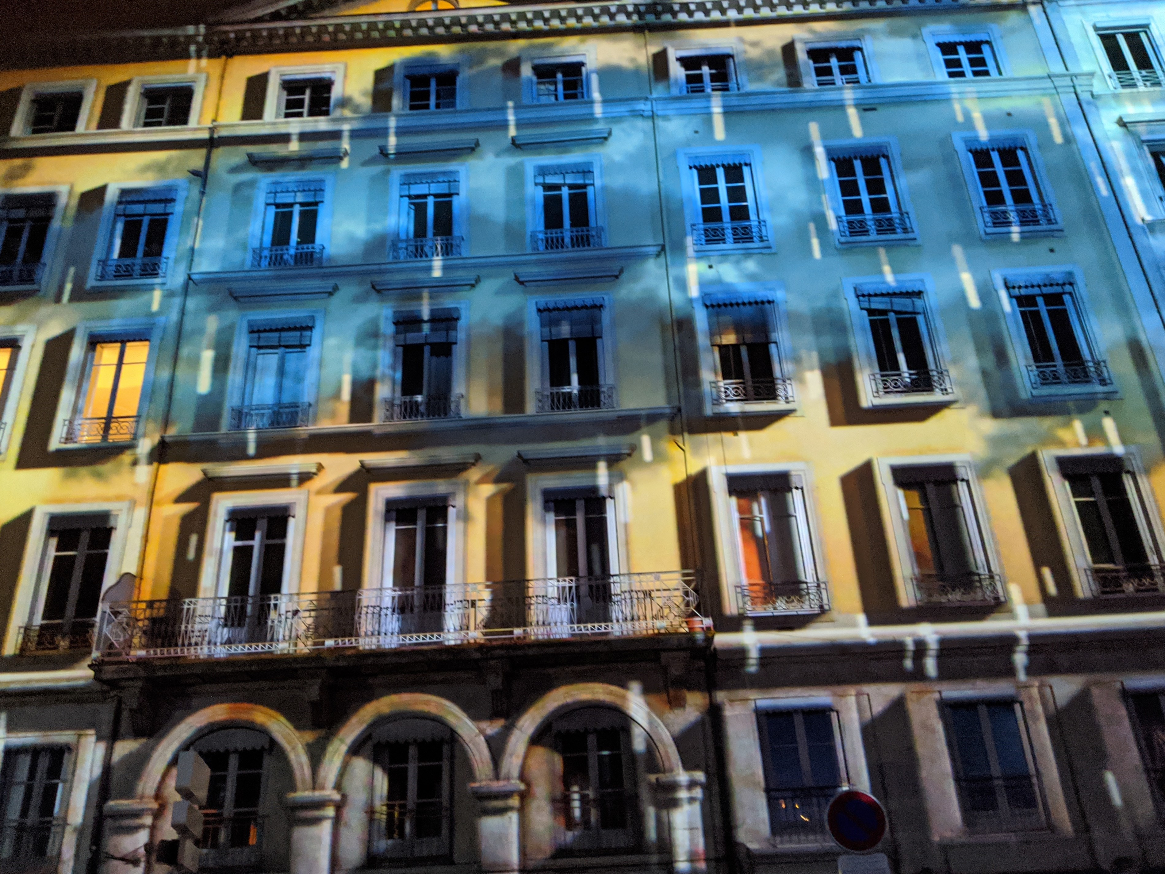
Facade
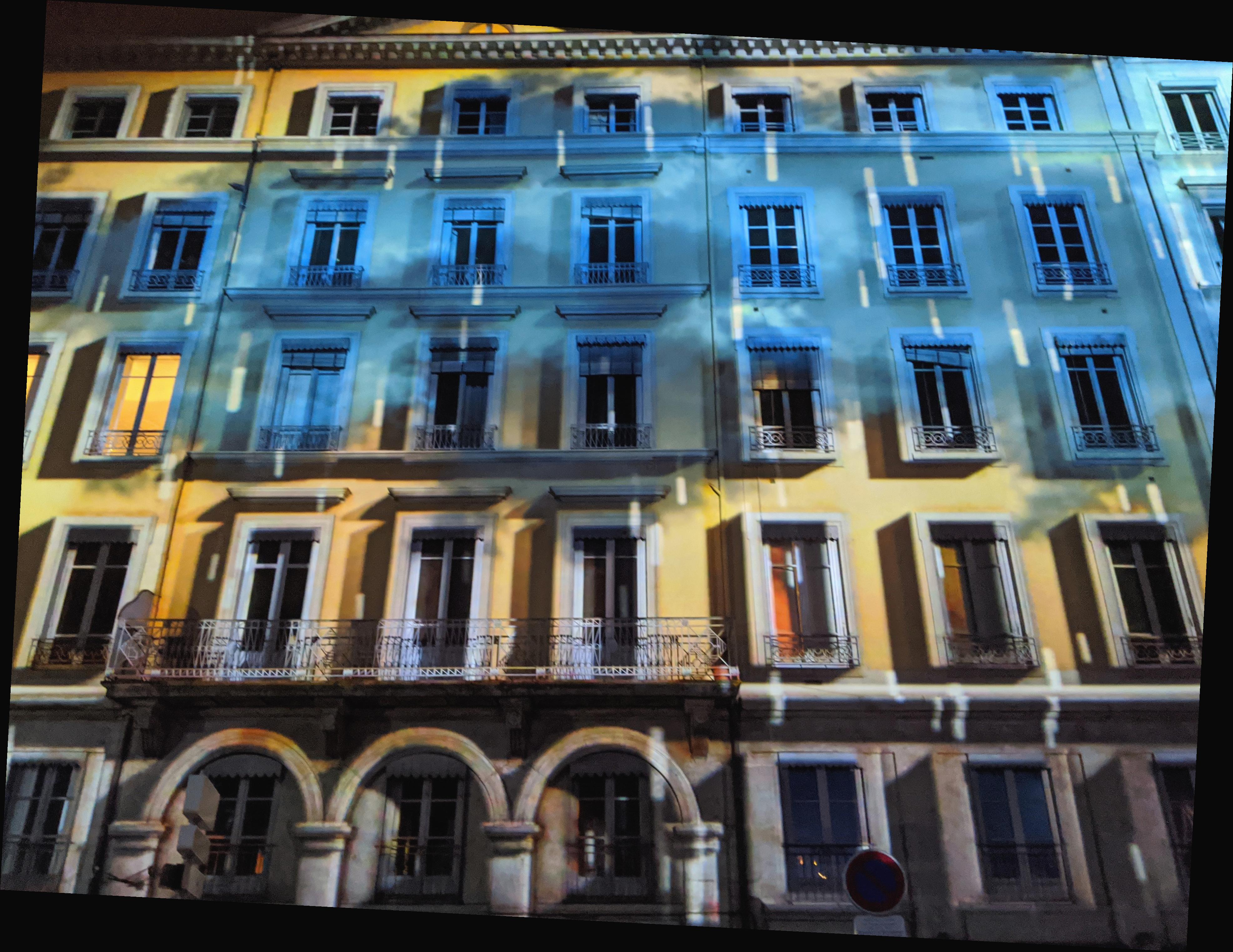
Facade after roation
Facade Histgram
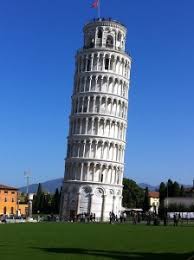
Pisa Tower
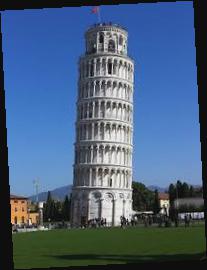
Pisa Tower after rotation
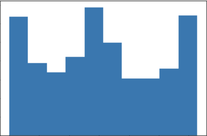
Pisa Tower Histgram

Chair
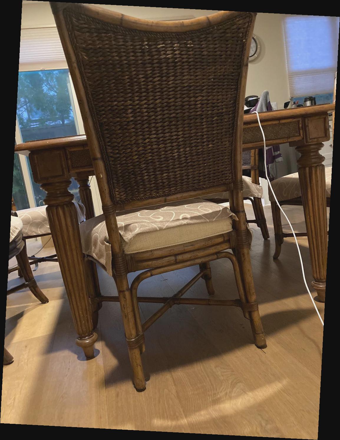
Chair after rotation
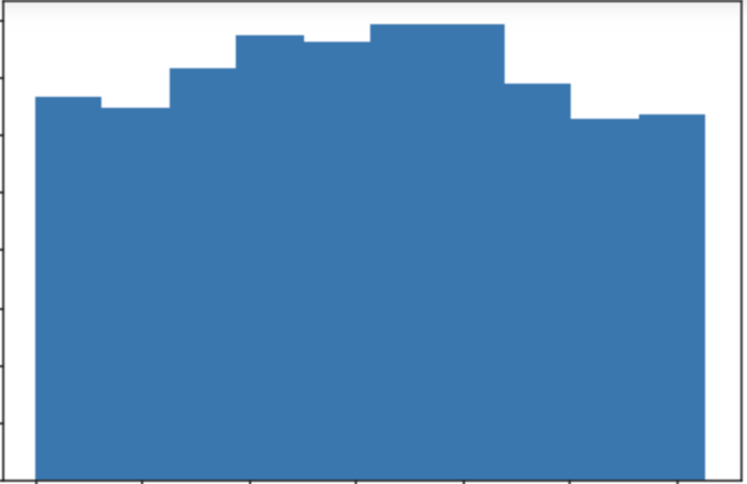
Chair Histgram

Failure Example
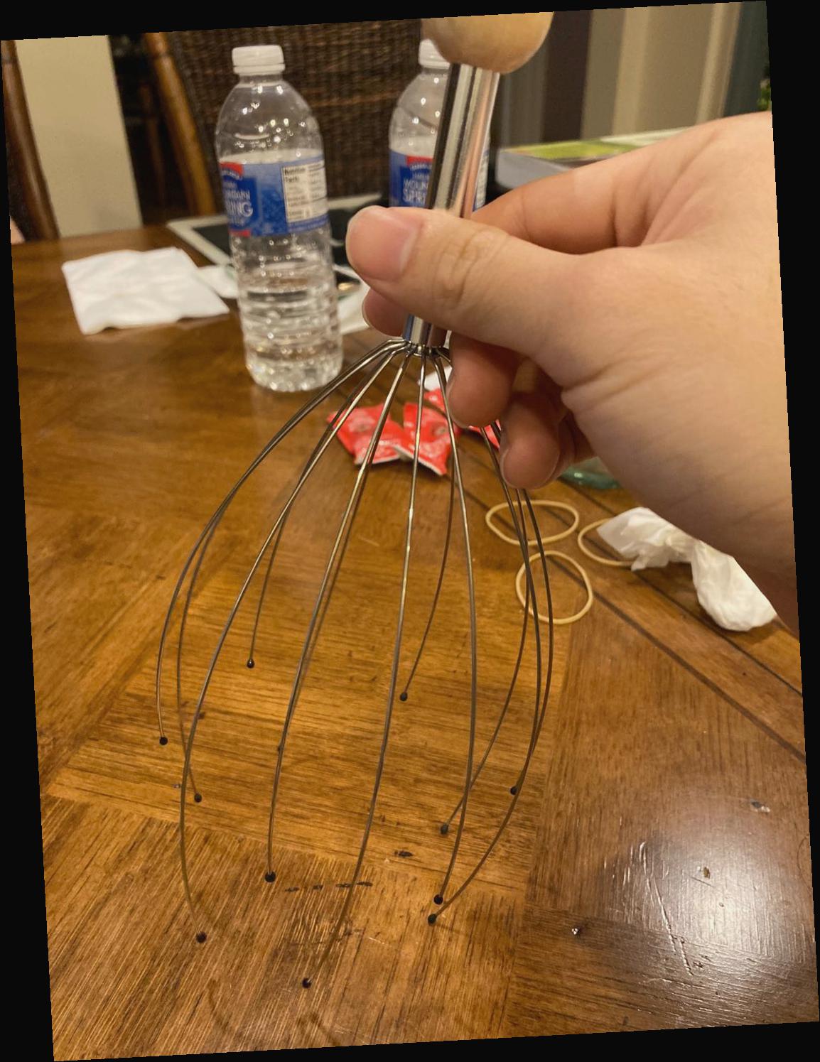
Failure Example after roation
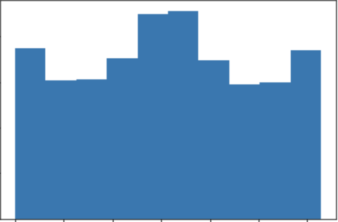
Failure Example Histgram
Image "Sharpening"
In this part, we did a "fake sharpeniing". What we did is that we compute the Gaussian filtered image, i.e., the blur image, subtract it from the original image. That leaves us only the high frequency part of the image. We choose an alpha value(by default I set it to be 3), as the amount that we will emphasise the high frenquency part of the image and add it back to the original image. We did not actually introduce any new variables, but visually we see the image with cleared edges.
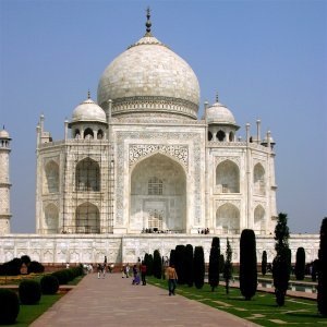
blur taj
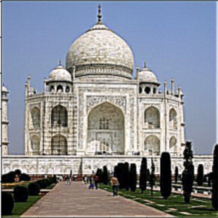
Sharpened taj

Blur money
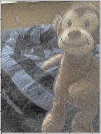
Sharp money
Resharpened blur camerman
Hybrid Images
Now in this part, we are doing the hybrid imaging. We first align two images. Next, we take the low frequency part of one image and the high frenquency part of the other images. Combing the two resulting in an image such that when we look at it closely, we saw one image and far away we see the other.
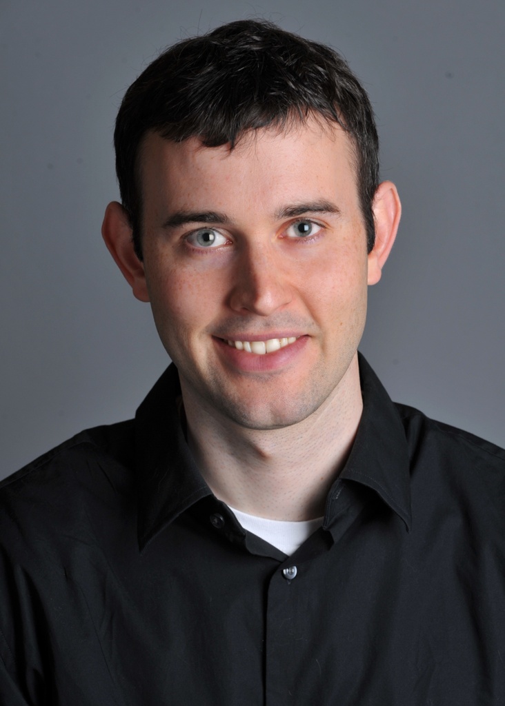
Derek Picture
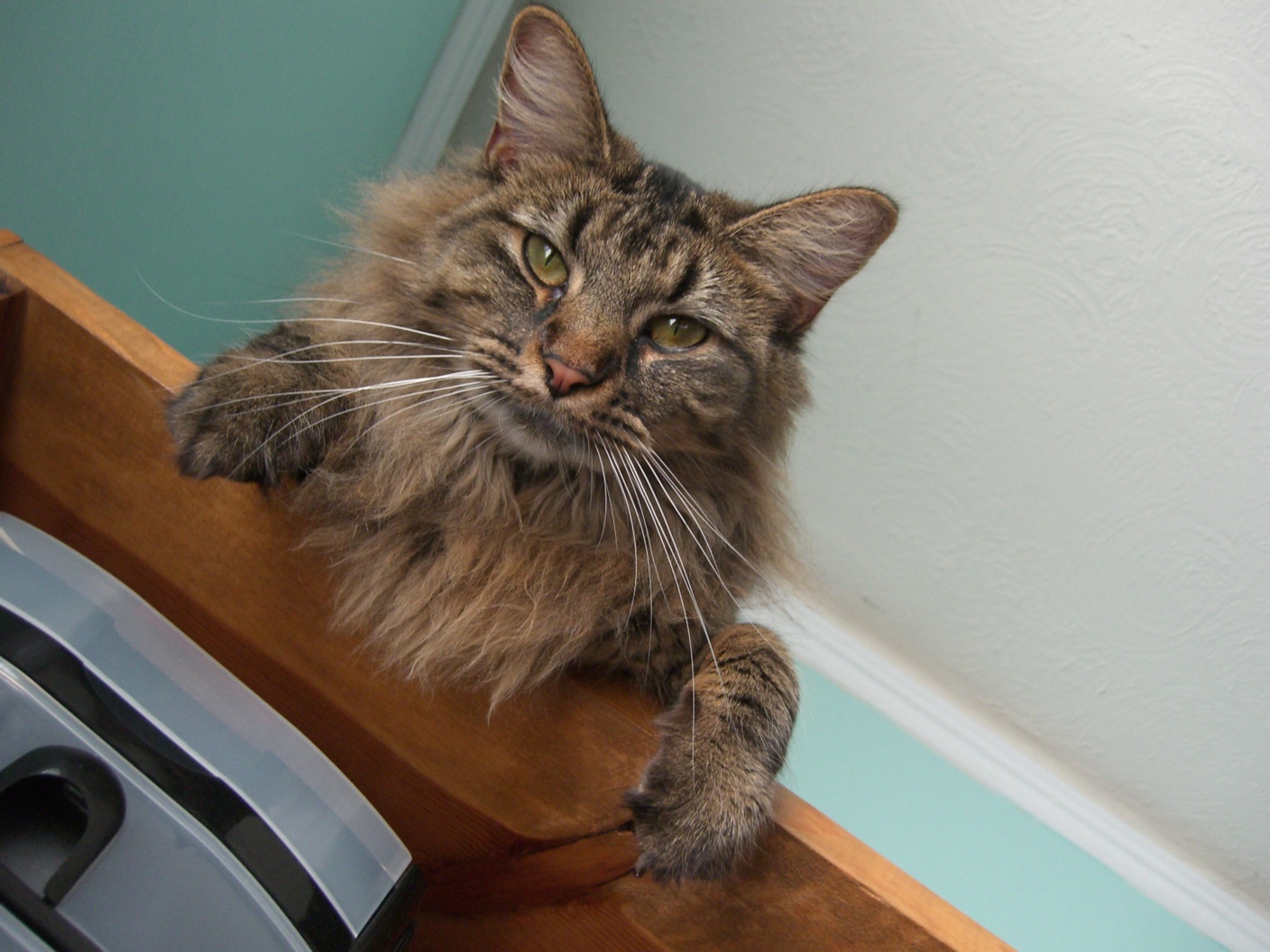
nutmeg Picture
Hybrid image of Derek and nutmeg

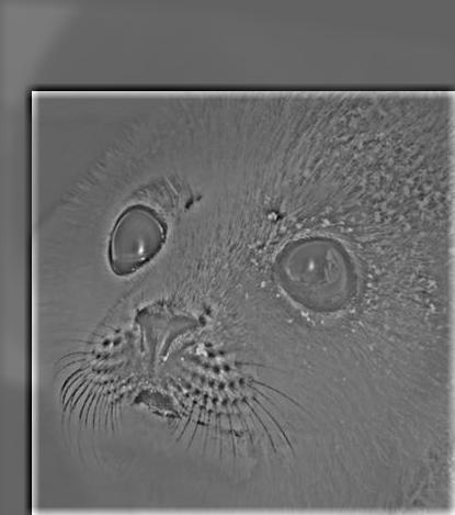
Successful seal image

Successful me image
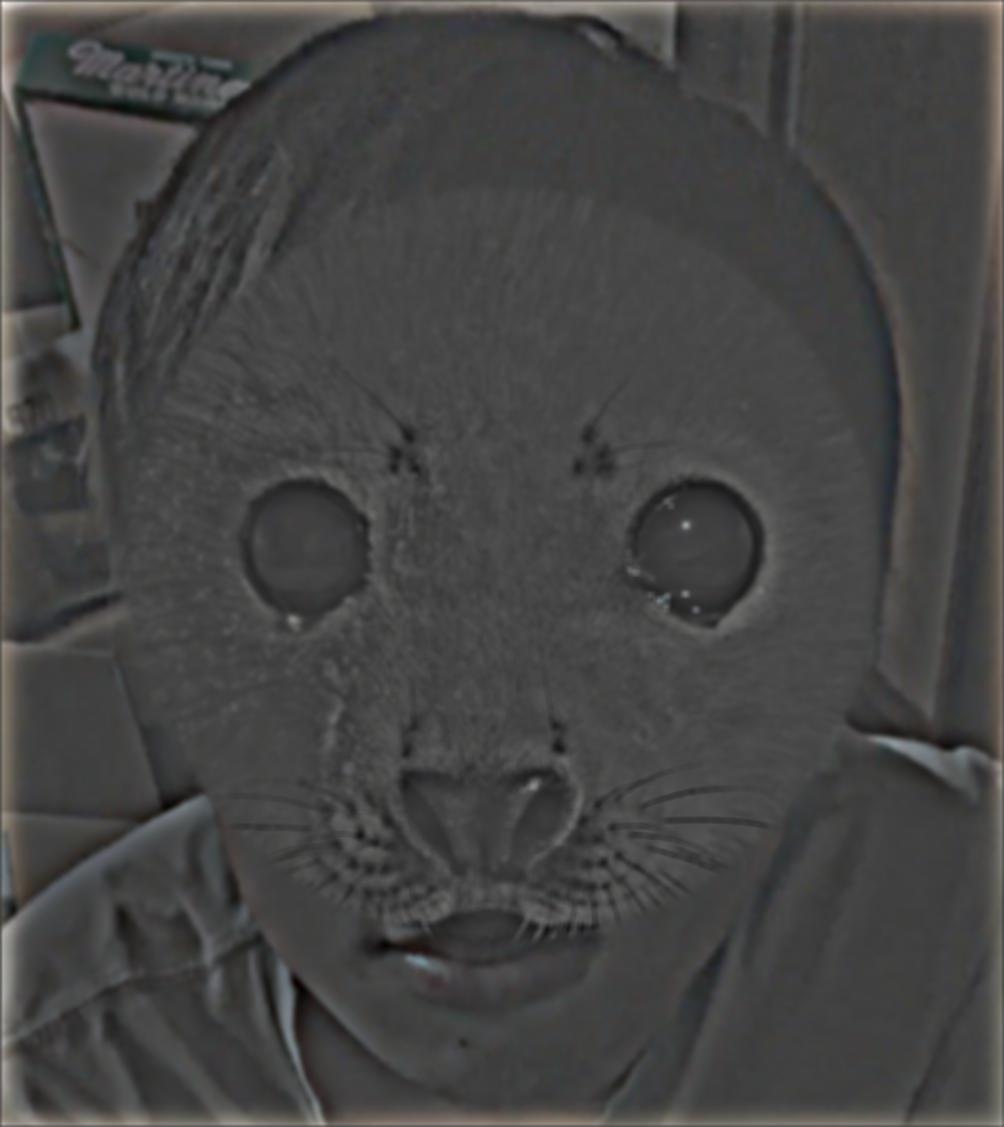
Successfuly hybrid of me and seal

fail example of seal

fail example of me
Failed hybrid
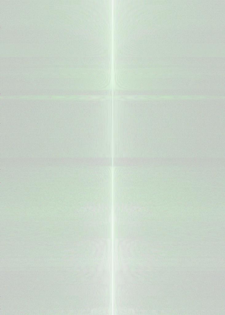
Fourier of DerekPicture
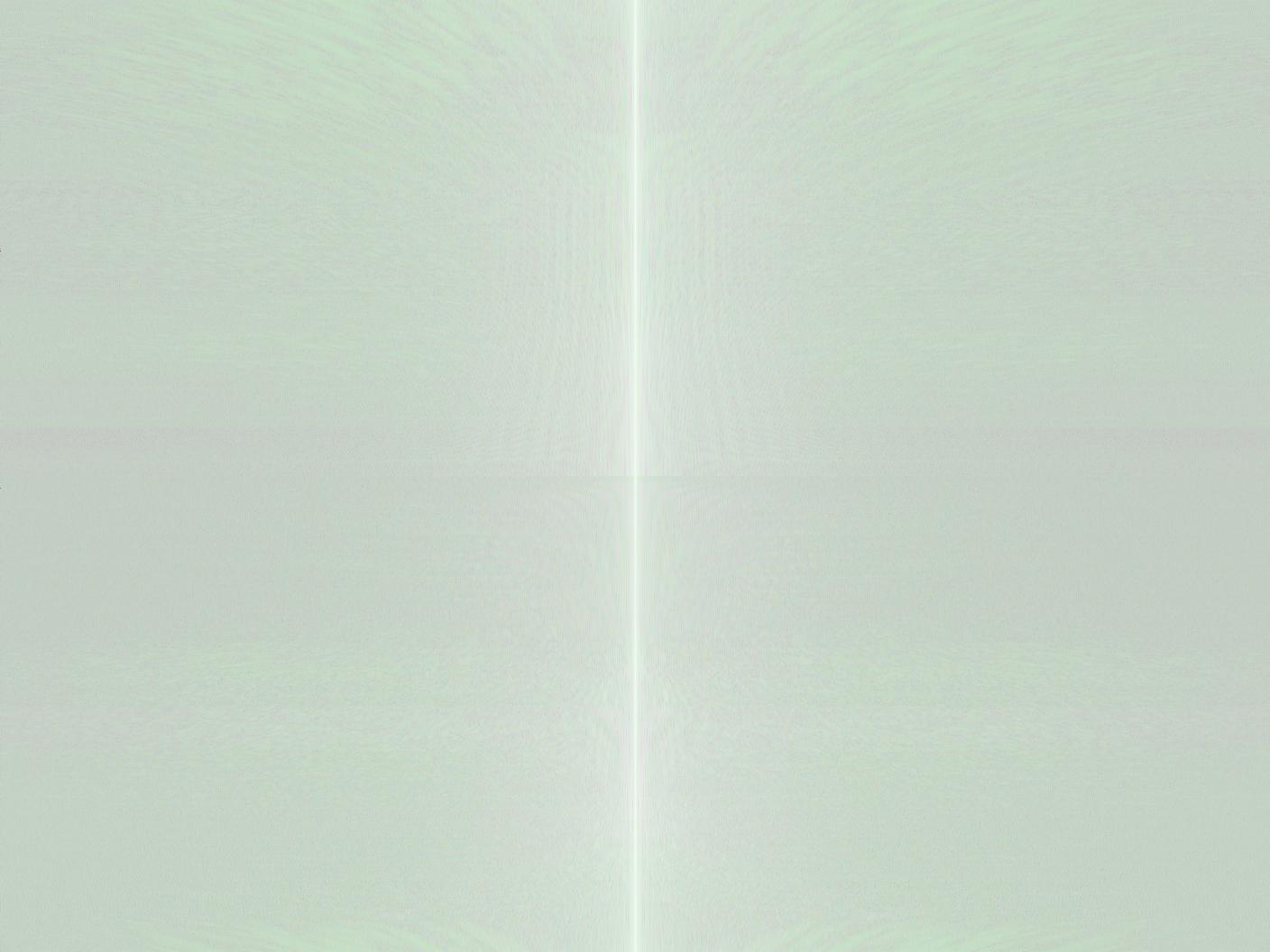
Fourier of nutmeg
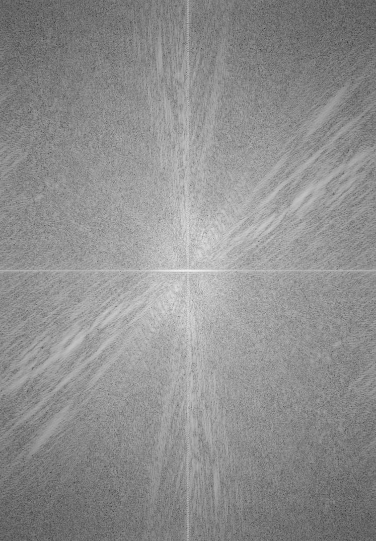
Fourier of high pass filter
Fourier of low pass filter
Fourier of the hybrid image
Gaussian and Laplacian Stacks
In this part, we find the gaussian stack and laplacian stack, which is preparing to use for next part. The Gaussian stack is basically the appling serveral times Gaussian filter to the same image, and put them into a stack. Laplacian stack, on the other hand, is the difference between the Gaussian filter and the origin, i.e. the high frenquency part. I also choose an image from the hybrid iamge part. As we can see, the Gaussian stack filter out one of the image, and the laplacian stack filtered out the other iamge I used to form the hybrid image. So this process can be imagine as the anti-processing of last part.
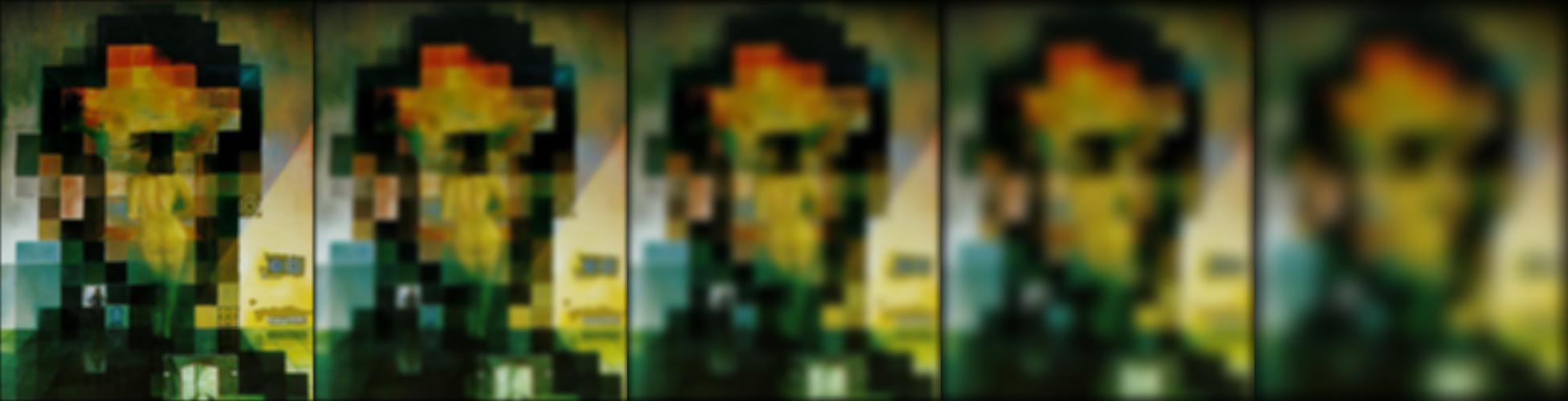
Gaussian Stack of Lincoin and Gala
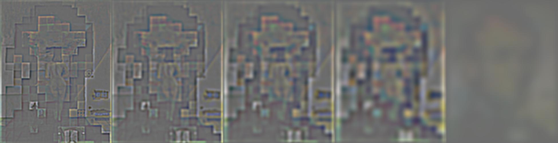
Laplacian Stack of Lincoin and Gala
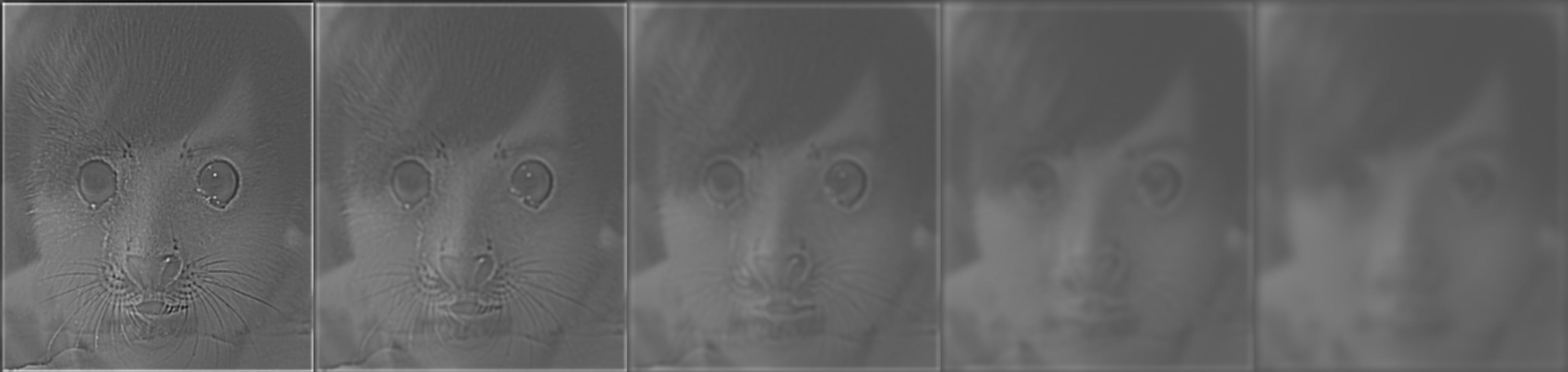
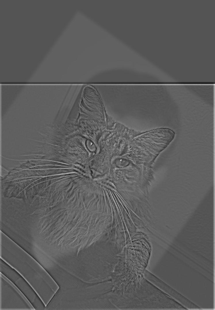
The Gaussian stack of the successful seal image from last part
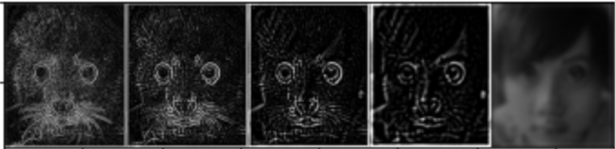
The Laplacian stack of the successful seal image from last part
Multiresolution Blending
In this part, we are trying to blend two images into one with a mask, and try to make the seam as vague as possible. The technique we are using is we need the laplacian stack and gaussian Stack from last part. We have the Gaussian stack of the mask and Laplacian stack for both of our image ready. In each layer, we mutiply the gaussian stack to one of the image's laplacian stack, and (1- gaussian stack) to the other image's laplacianstack. Lastly, we sum over the blend stack and get the image. The mask I used to combine apple and orange and water and fire is the mask where half of it is white and half of it is black (half 1's and half 0's). In addition, I make a circle mask where the center part is 0's and the corner are 1's. By that, I can put my face into a seal, which is the images from part2.2.

Apple

Orange
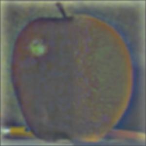
Apple Orange blend into one
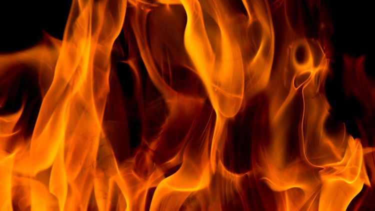
Fire
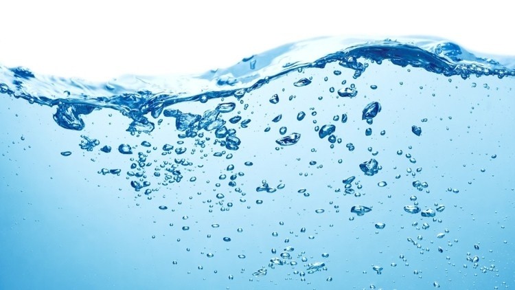
Water
Fire Water blend into one
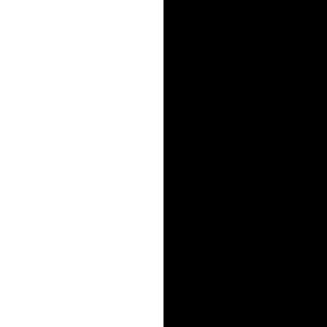
The orap mask
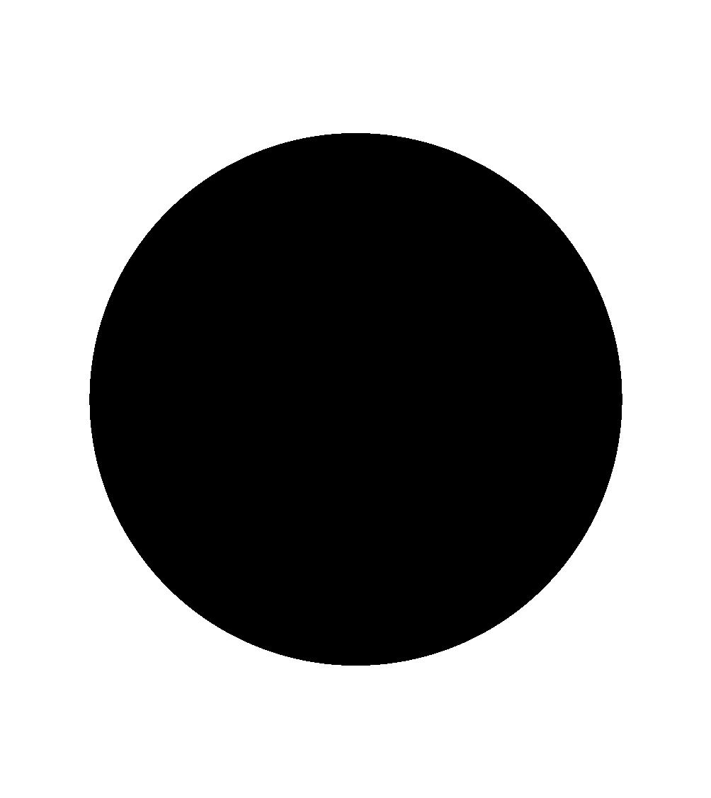
The circle mask
Me and seal blend into one (same image from part 2.2)
Conclusion
In this project, what I think is the most important things to learn is the usage of filtering. Clearly, the power of Gaussian filter can help us do a lot of interesting things with images. Worth to mention, one improvement that can possibly made to my project is the blending part and the auto-rotation. For some reason,the colored images all looked very dark. It might be caused from the coversion loss of images. For the auto-rotaion, some of the angles seemed to be hard to detect with my algorithmn.