Fun with Filters and Frequencies!

CS 294-26 • Fall 2020 • Project 2

Shubha Jagannatha

Overview

In this assignment, I create several filters and effects by utilizing and modifying the frequency distribution of these images!

Part 1

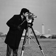
Part 1.1: Finite Difference Operator

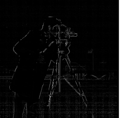
In this portion of the project, our aim was to get to a binarized edge image. We accomplished this by finding the partial derivative of the image in the x and y directions by convolving the image with the finite difference operators D_x = [[1, -1]] and D_y = D_x transposed. Doing so would give us the "edges" moving in the x direction and y direction. Then, we find the gradient magnitude from the square root of the sum of D_x and D_y squared. 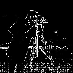This would give us the magnitude of all edges combined in a single image. Lastly, we "binarized" the images by using a chosen threshold (0.1 in the case shown) by turning any value > threshold into 1 and any value <= threshold into 0. As one can see, the final edge image has a significant amount of noise.

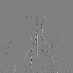
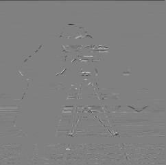
Original Image	D_x Image	D_y Image
Gradient Magnitude Image	Edge Image Image

Part 1.2: Derivative of Gaussian (DoG) Filter

In this portion of the project, we want to remove the noise previously seen in part 1.1 by blurring the original image, equivalent to convolving it with a Gaussian. We tried two methods to achieve this.

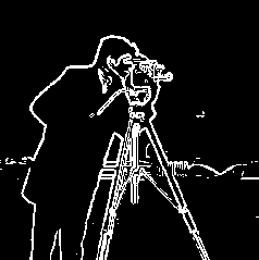
The first (naive) method we used to blur the image was to blur the image by convolving it with a 2D gaussian, then getting the D_x image, the D_y image, the gradient magnitude image, and the edge image as we did in the previous part. Here is the final result with noticeably reduced noise, especially towards the bottom half of the image. The edges also appear stronger here.

Naive Result

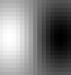
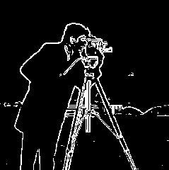
The second, more advanced method would be to achieve the same result with a single convolution instead of two by creating a derivative of gaussian filter. In order to do this, we can convolve the gaussian by itself with the D_x and D_y filter to create the derivative of gaussian (DoG) filter and do a single convolution with the image and the DoG filter. Here are the resulting DoG filters as images and the final result. The final result is the same as our naive result with any slight differences caused by the mode used for convolution.

D_x filter

D_y filter

Final Result

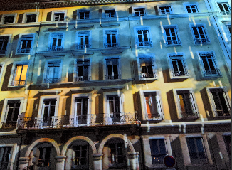
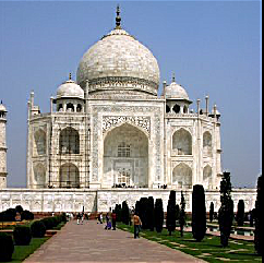
Part 1.3: Image Straightening

For this part, we would like to take in an image and automatically straighten it. Since most images have a preference for vertical and horizontal edges due to gravity, we essentially want to check whether our edges are close to 0, 90, 180, and 270 degrees. In order to do this, I tested a number of rotations from -10 to 10 degrees for each image and chose whichever rotation had the maximum count of vertical or horizontal edge pixels.

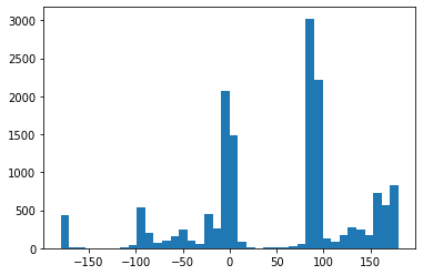
Here are the results and histogram for a number of images:

Facade

Before	Histogram
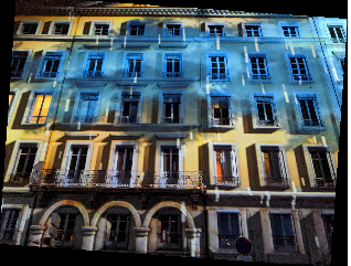
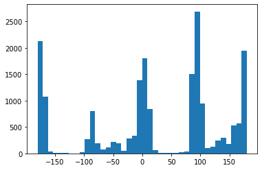
After: Rotated -4 Degrees	Histogram

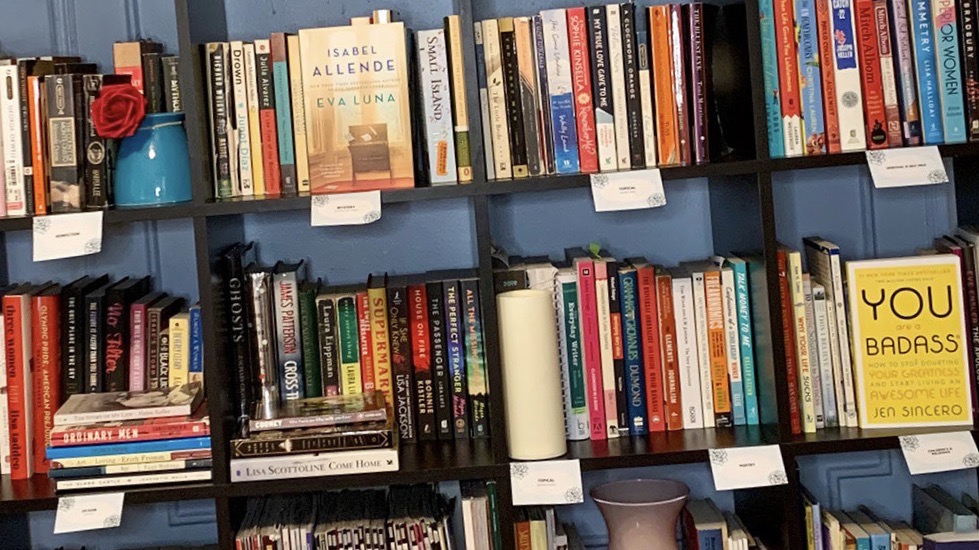
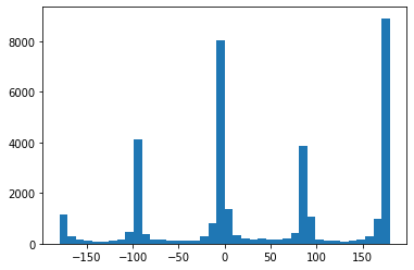
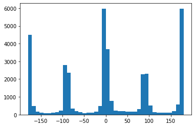
Books

Before	Histogram
After: Rotated -6 Degrees	Histogram

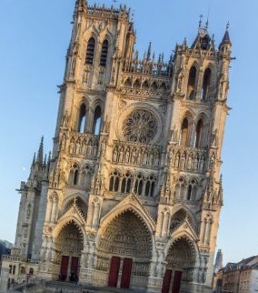
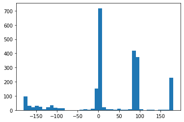
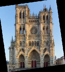
Cathedral

Before	Histogram
After: Rotated 8 Degrees	Histogram

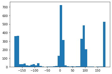
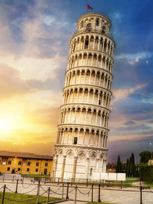
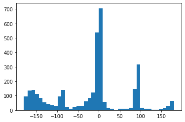
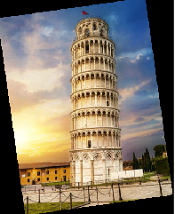
Failure Case: Leaning Tower of Pisa

Here's a case where the straightening didn't work as well because with the leaning tower of Pisa, the assumption that majority of the edges are vertical or horizontal no longer holds.

Before	Histogram
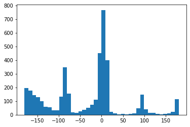
After: Rotated 8 Degrees	Histogram

Part 2

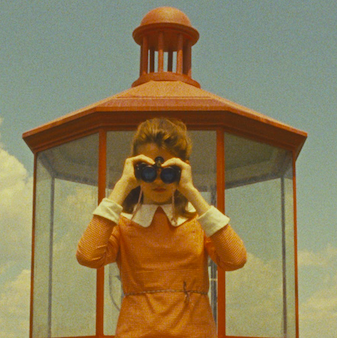
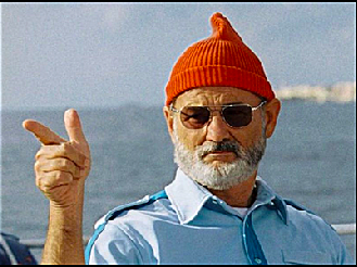
Part 2.1: Image "Sharpening"

In this portion of the project, we are sharpening images by creating a version of the image with only the high frequencies and adding it back into the image. We do this by taking the original image, creating a blurred version (with only the low frequency elements in the image), and subtracting the blurred version from the original image to only have the high frequencies remaining. In my code, I've combined all of these operations into a single convolution operation called the unmask filter. Here are some examples of sharpened images:

Before	After
Before	After
Before	After

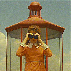
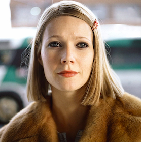
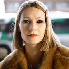
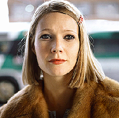
The images I pulled from Wes Anderson films have some amount of grain in them originally. This high frequency noise is amplified by the sharpening. Here is an image I've blurred and resharpened. I notice that there are some artifacts which showed up after blurring the image (particularly by her chin and her hair frizz) which is still present when I resharpen the image. A lot of the detail from the original image is lost when blurring and resharpening:

Original

Blurred

Resharpened

Part 2.2: Hybrid Images

Here I've successfully created hybrid images by taking two images, aligning and cropping them, running a high pass filter on one, running a low pass filter on the other, and overlaying the two images. When the viewer is close to the image, they see primarily the high frequency elements and when they are further away or blur their vision, they primarily see the low frequency elements. This allows viewers to see two different pictures in the same image! 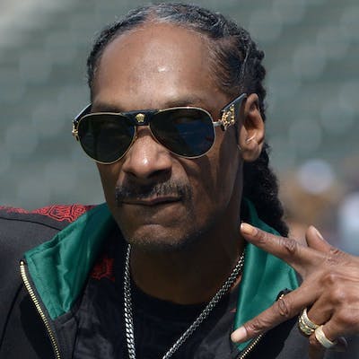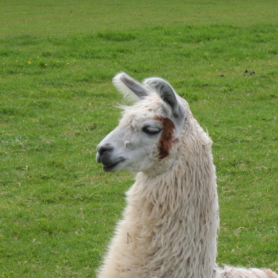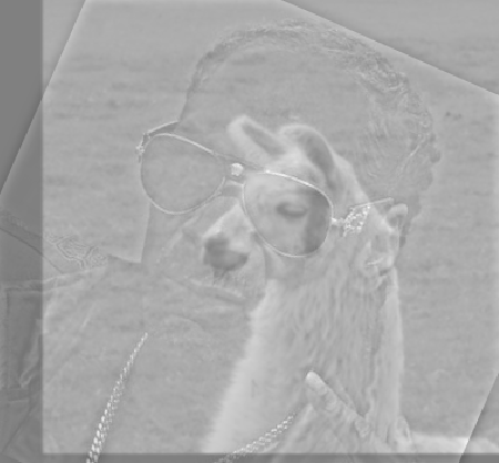These images do have to have some means of alignment, or we arrive at the failure case demonstrated below (Snoop Llama). The lack of alignment makes the two images very distinguishable as separate images and breaks the hybrid image illusion.

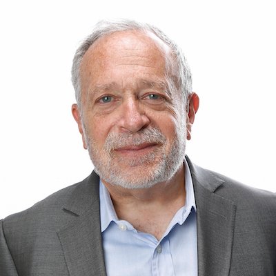
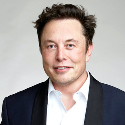
Robert Reich	Elon Musk	Robert Musk
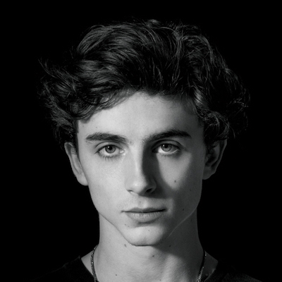
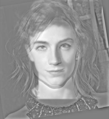
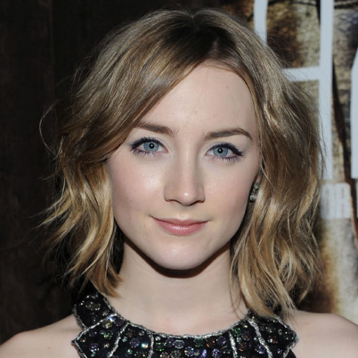
Timothee Chalamet	Saorise Ronan	Timothee Ronan
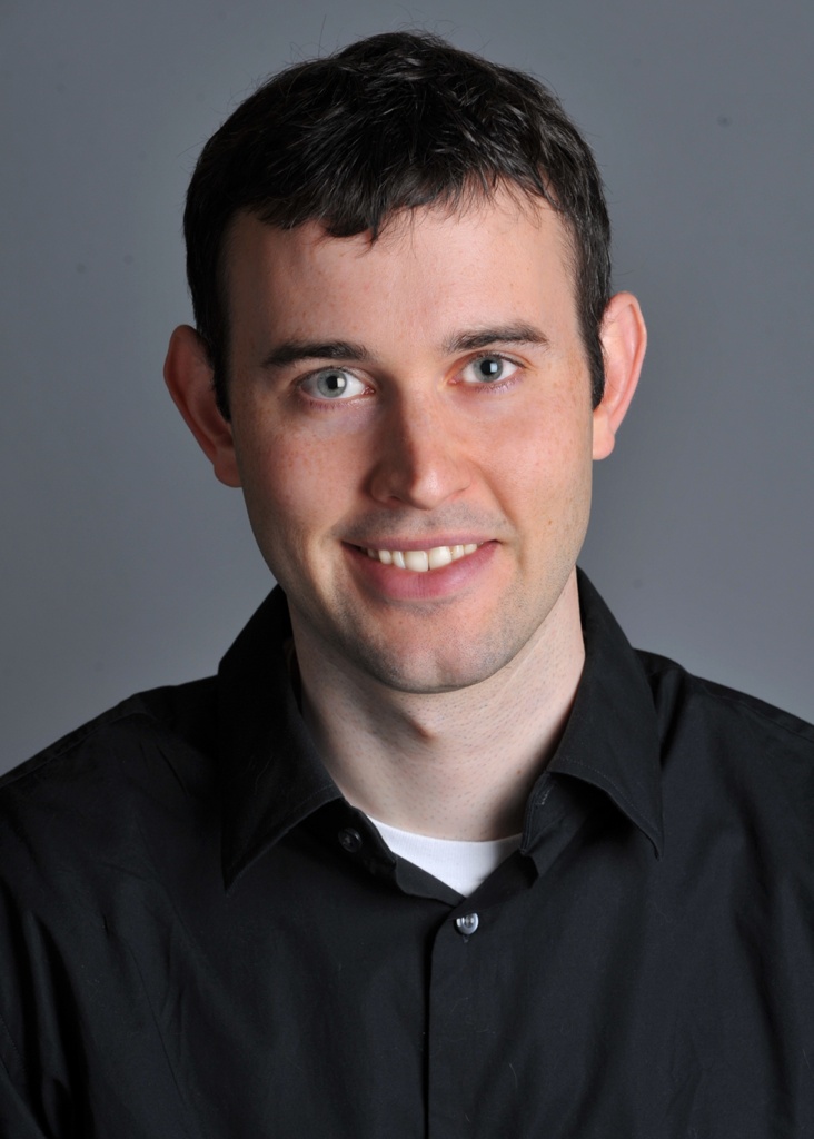
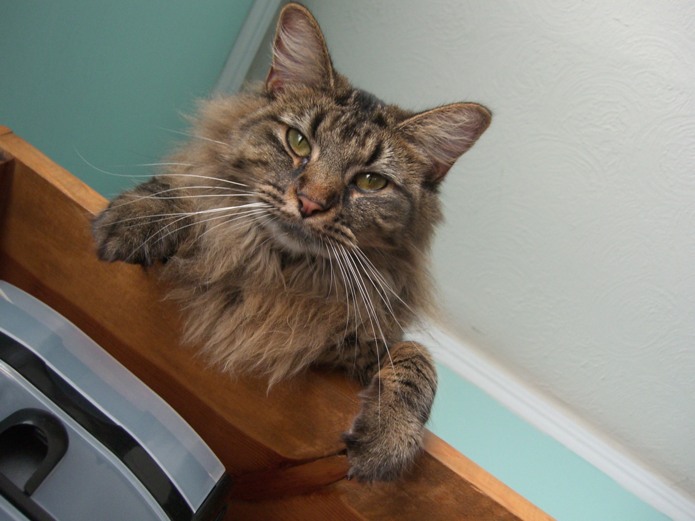
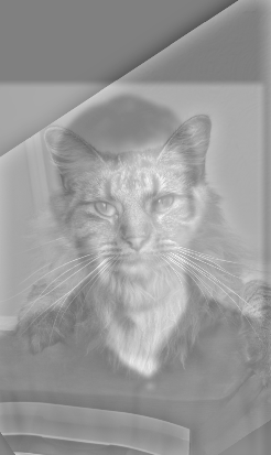
Derek	Nutmeg	Dermeg
Failure Case: Snoop Dogg	Failure Case: Llama	Failure Case: Snoop Llama

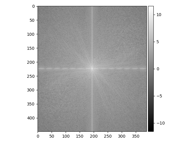
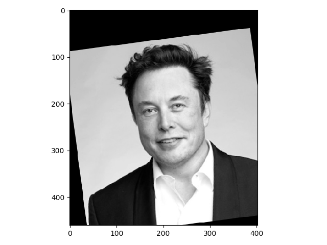
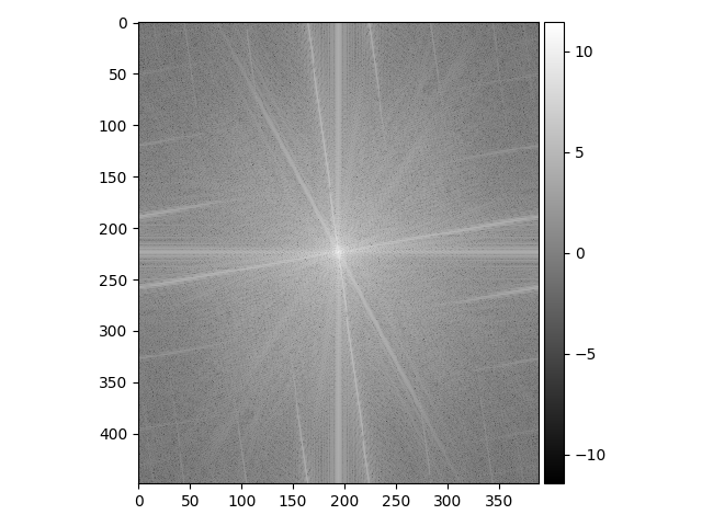
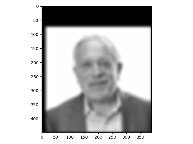
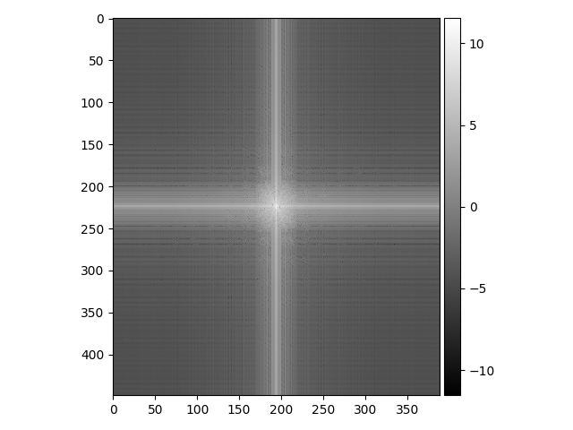
Here is the breakdown of the Robert Musk hybrid image process in the fourier domain.

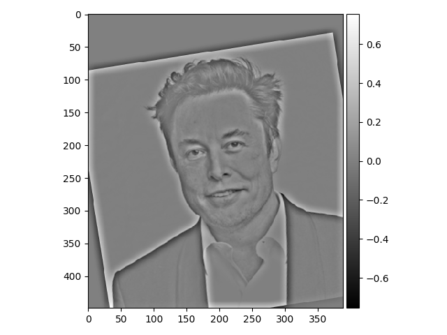
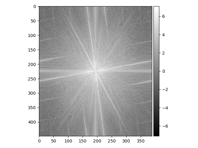
Reich	Reich: Fourier Domain	Musk	Musk: Fourier Domain
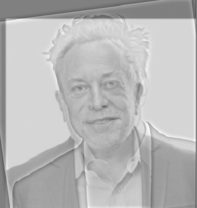
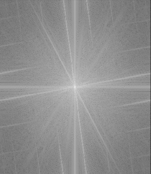
Reich: Lowpass	Reich: Lowpass Fourier Domain	Musk: Highpass	Musk: Highpass Fourier Domain

Hybrid Image

Hybrid Image Fourier Domain

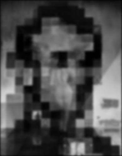
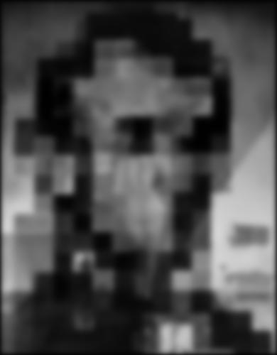
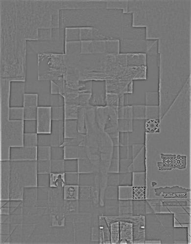
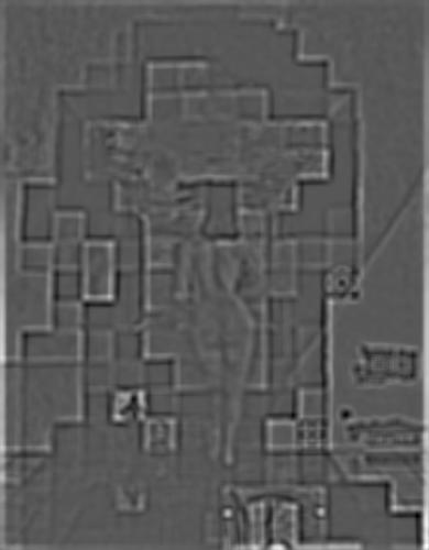
Part 2.3: Hybrid Images

In this portion of the project, I created a Gaussian and Laplacian stack.

The Gaussian stack was created by repeatedly applying a gaussian of kernel size = 9 and sigma = 3 to the previous image on the stack. The Laplacian stack was created by subtracting the neighboring images in the Gaussian stack. The first row here is the Gaussian stack and the second row is the Laplacian stack.

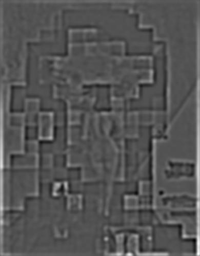
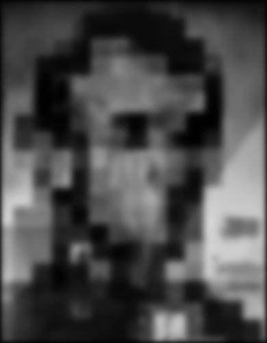
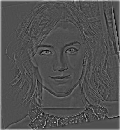
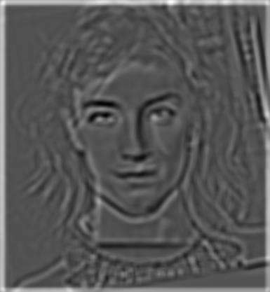
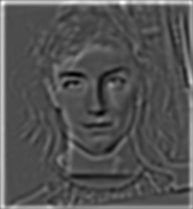
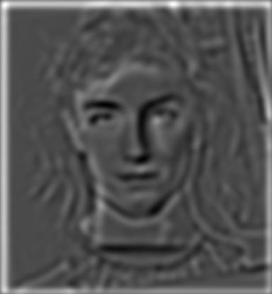
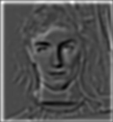
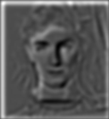
Here's a Laplacian stack of m Timothee Chalamet + Saorise Ronan image to show the different frequencies.

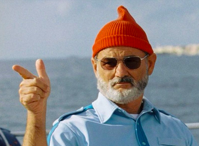
Part 2.4: Hybrid Images

In this last part of the project, I've blended two images using a mask. In order to accomplish this, I created Laplacian pyramids for the two images and a Gaussian pyramid for the mask. Then I combined the two Laplacian pyramids into a third hybrid Laplacian pyramid by using the gaussian pyramid of the mask as weights. Lastly, I summed up the images in the Laplacian pyramid to obtain the final image.

Here are some of my final results!

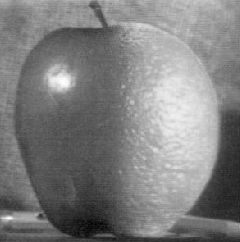
Apple	Orange	Mask	Orapple
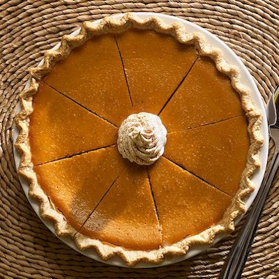
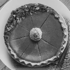
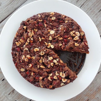
Pie	Cake	Mask	Pie Cake
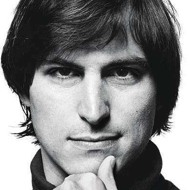
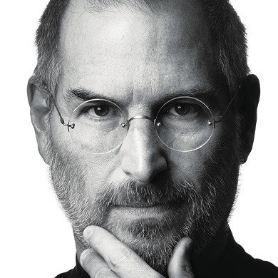
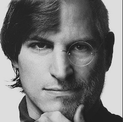
Young Steve	Old Steve	Mask	Combined Steve

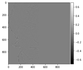
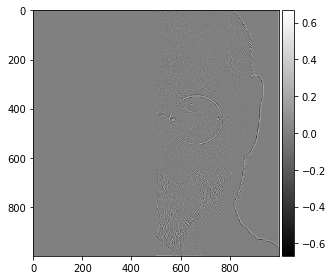
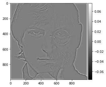
Here's a couple examples of the high frequency and low frequency combined images:

Young Steve, High Freq	Old Steve, High Freq	Combined, High Freq
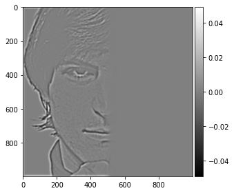
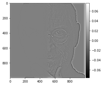
Young Steve, Low Freq	Old Steve, Low Freq	Combined, Low Freq

That's all for this assignment. I particularly enjoyed the creation of hybrid images and seeing the frequency breakdown shown through the Laplacian pyramid!