Project 2: Fun with Filters and Frequencies!
Roshni Rawal
CS 194-26 Fall 2020
September 27, 2020
Part 1.1: Finite Difference Operator
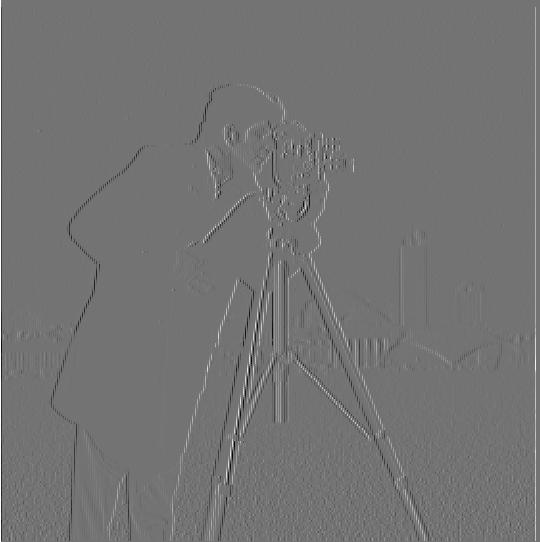
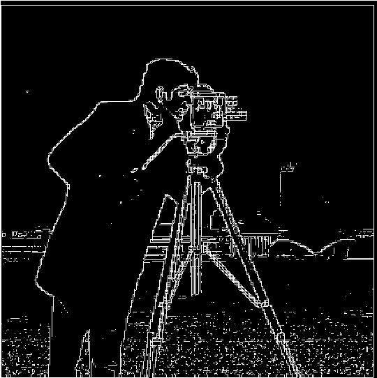
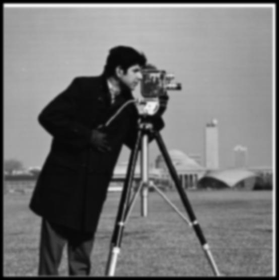
For part 1.1, we detected the edges in our image by using the gradient magnitude of the image. We first computed the convolution of our image with vectors [[1, -1]] and [[1][-1]], the former being the partial derivative in the x direction (since we are taking the difference between pixels in the x direction), and the latter being the partial derivative in the y direction. To calculate the edge strength of the edges in the image we used the gradient magnitude, or sqrt((df/dx)^2 + (df/dy)^2) at each pixel, which tells us the steepness of the slope at each pixel. From there we defined some threshold for which if the gradient magnitude value was larger than the threshold, we determined that the pixel was an edge. For the image below, we used the threshold alpha=0.13.
Finite Gradient Images
Image 1 is the x gradient.
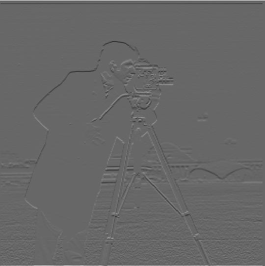
Image 2 is the y gradient.
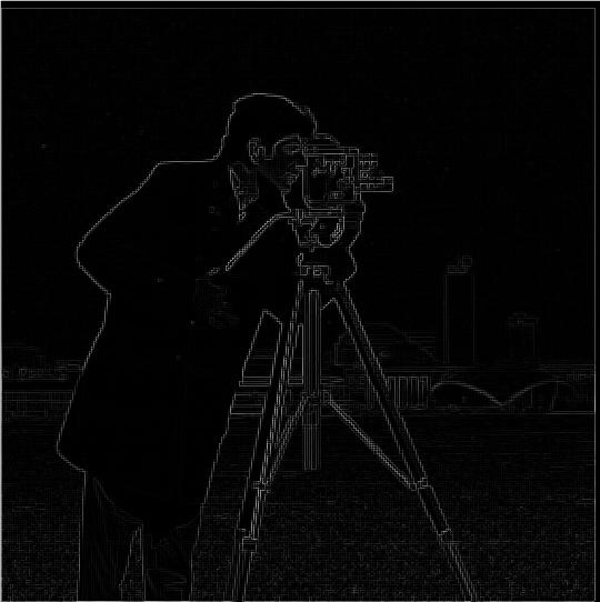
Image 3 is the gradient magnitude.
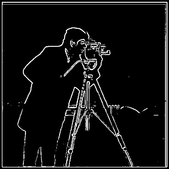
Image 4 is the edge image binarized.
Part 1.2: Derivative of Gaussian(DoG) Filter
For part 1.2 we first blurred our image by convolving it with a gaussian kernel (of size=15, sigma=1) and then computed the binarized gradient magnitude image like we did in part 1.1. Notice that much of the noise that was in our edge image in part 1.1 has disappeared and we are able to see the cameraman clearly.
DoG Images
Image 1 is the blurred image.
Image 2 is the new edge image.
Image 3 is the DoG filter image for d_x.
Image 4 is the DoG filter image for d_y.
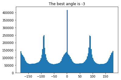
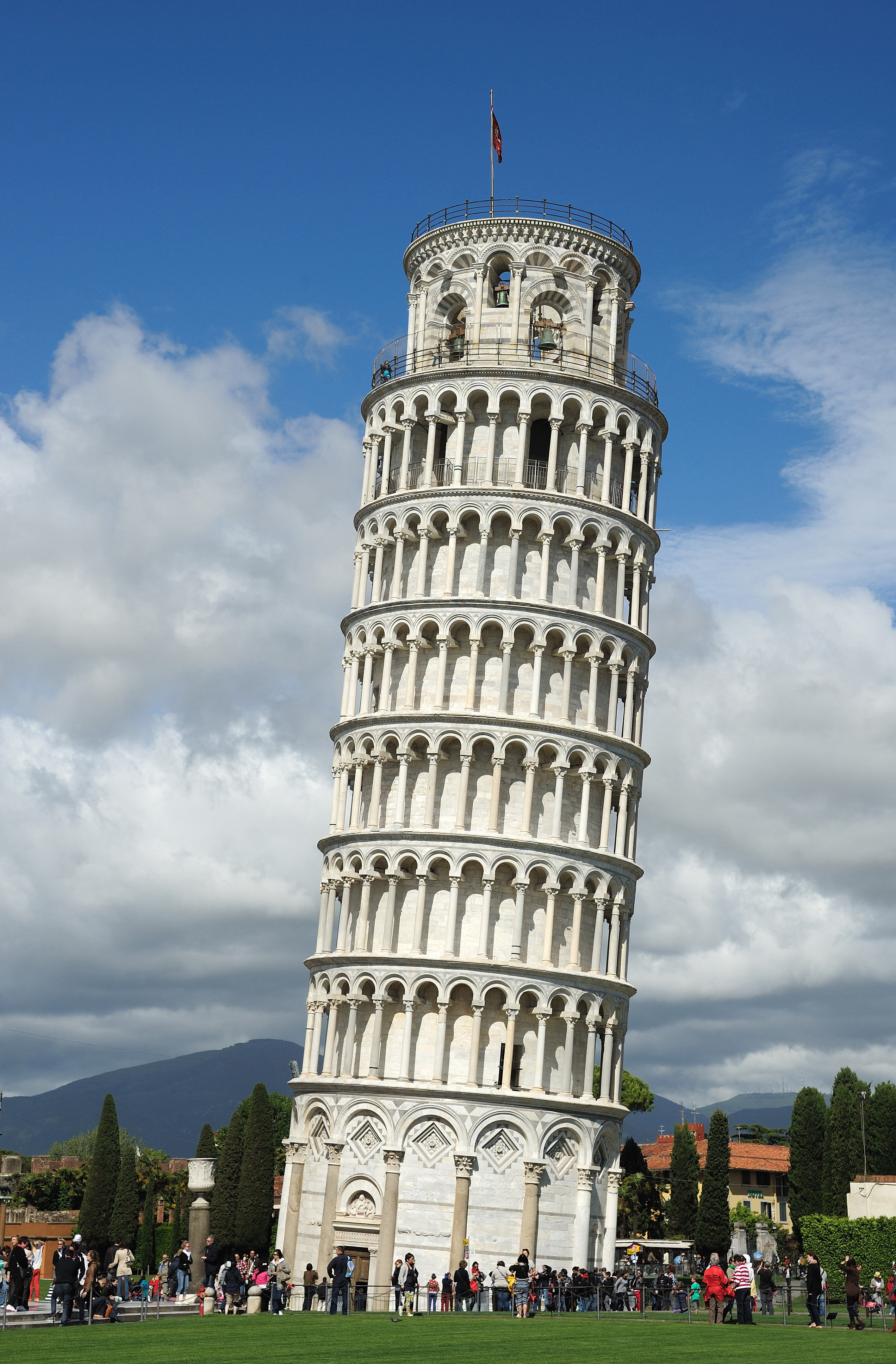
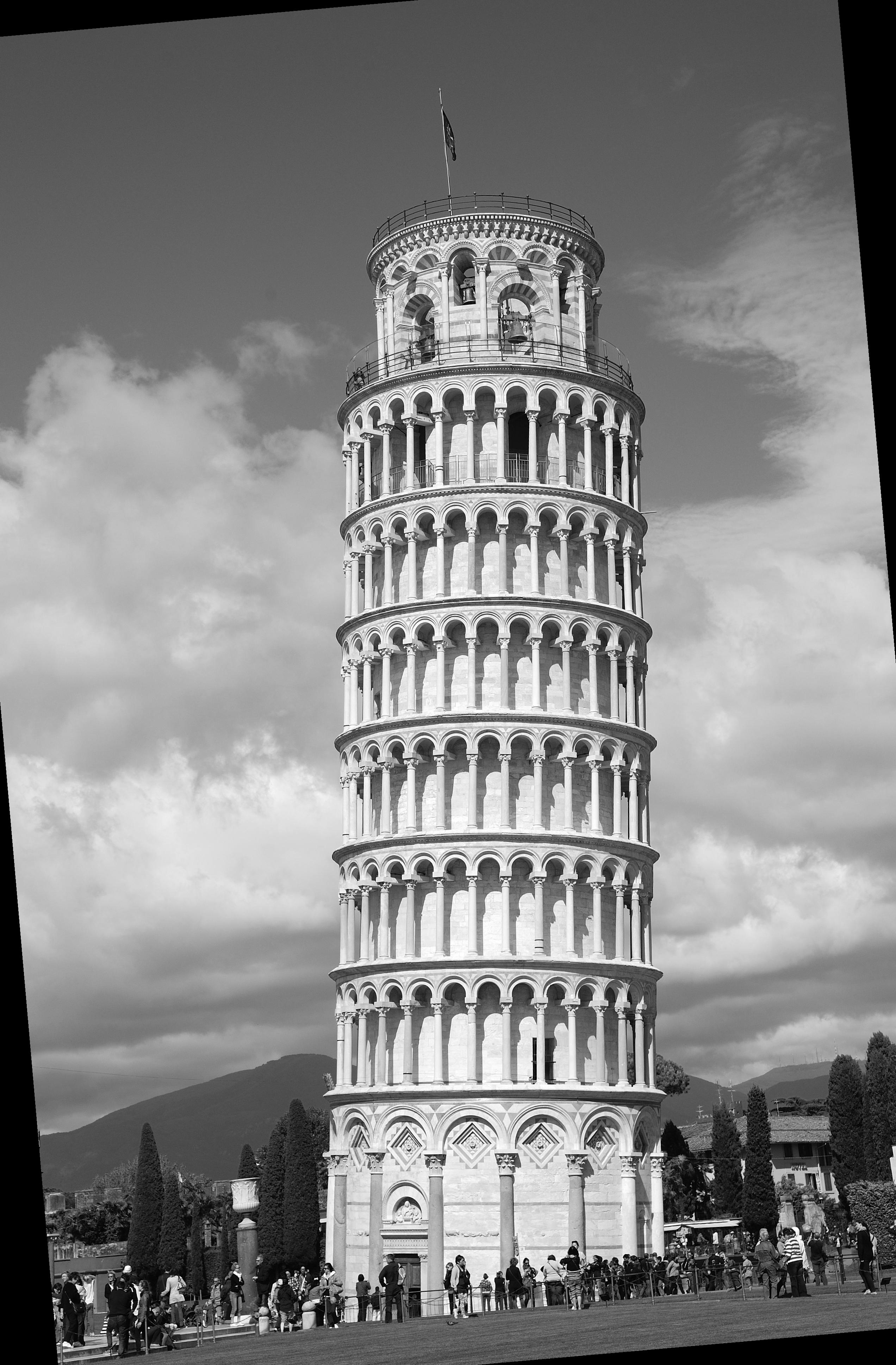
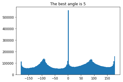
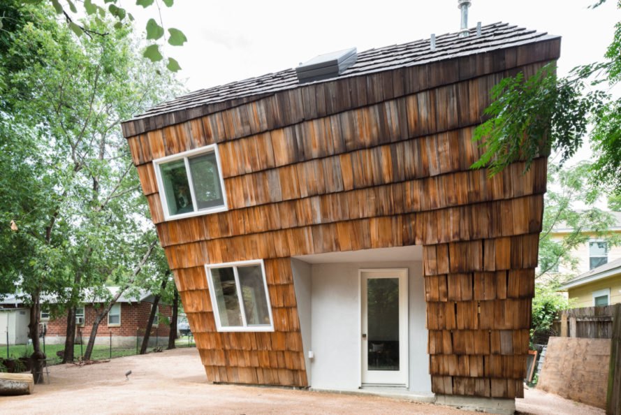
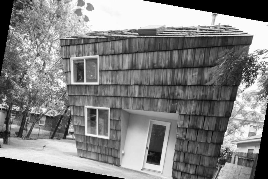
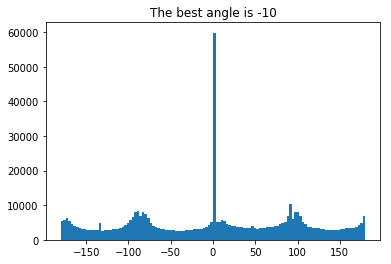
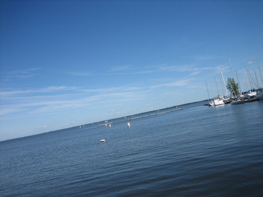
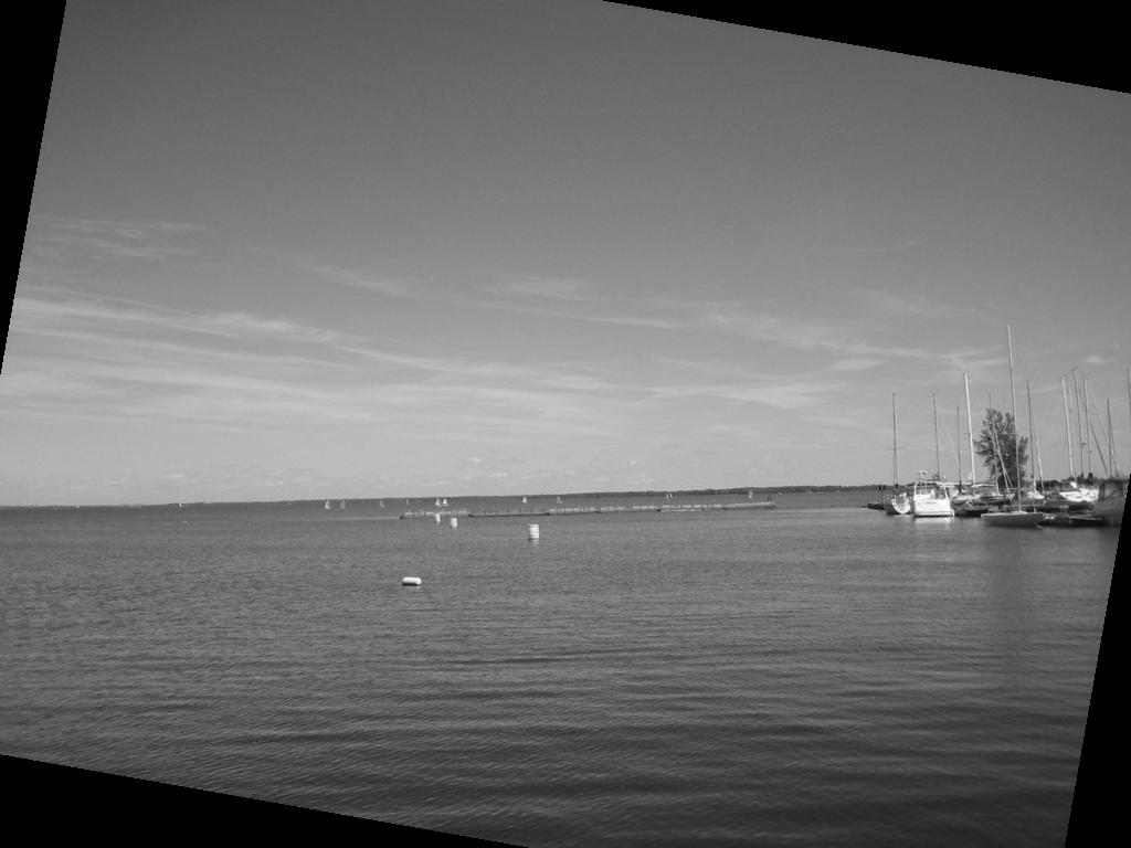
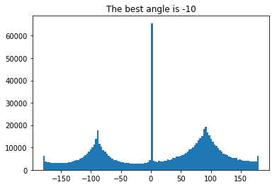
Part 1.3: Image Straightening
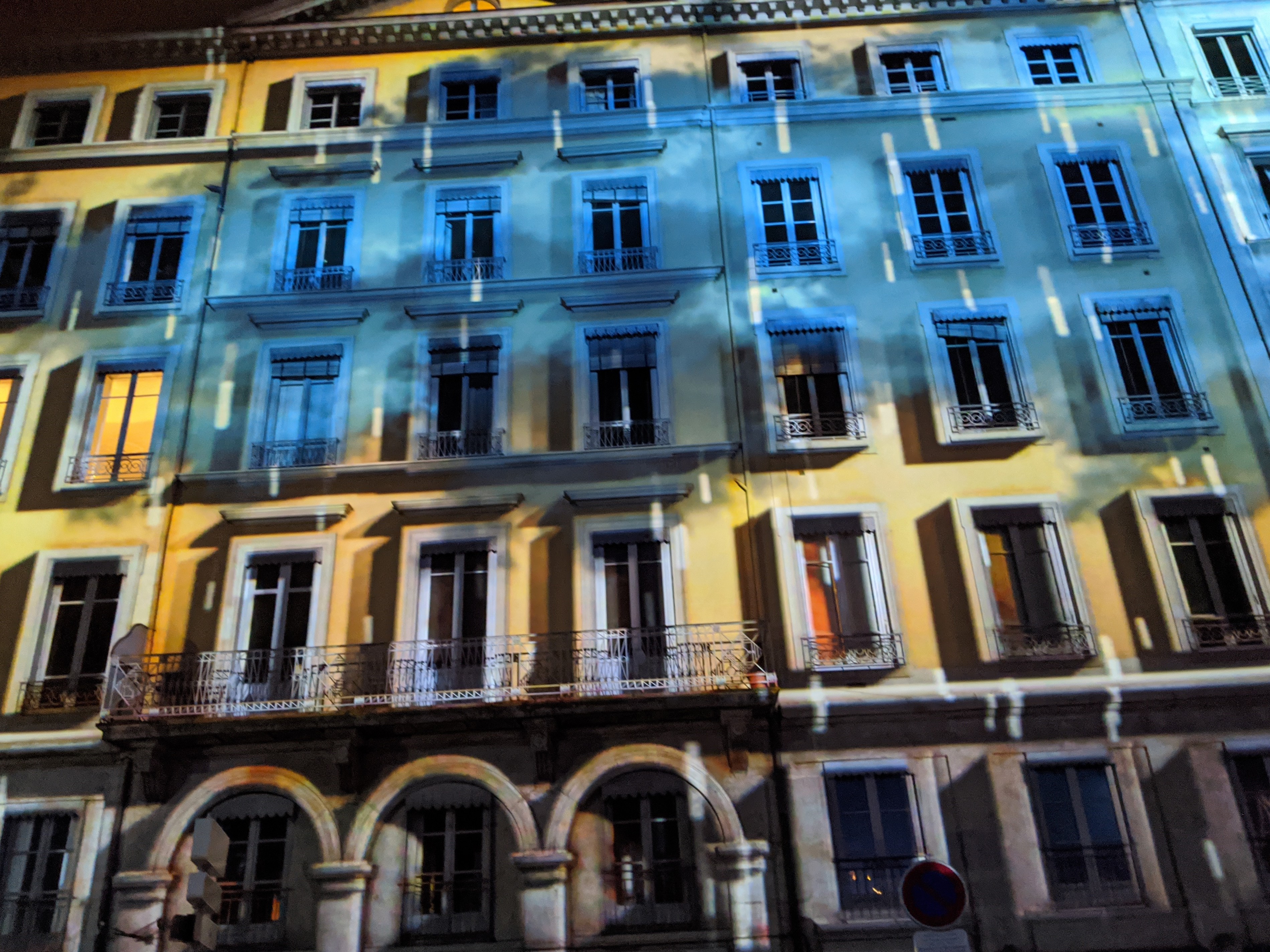
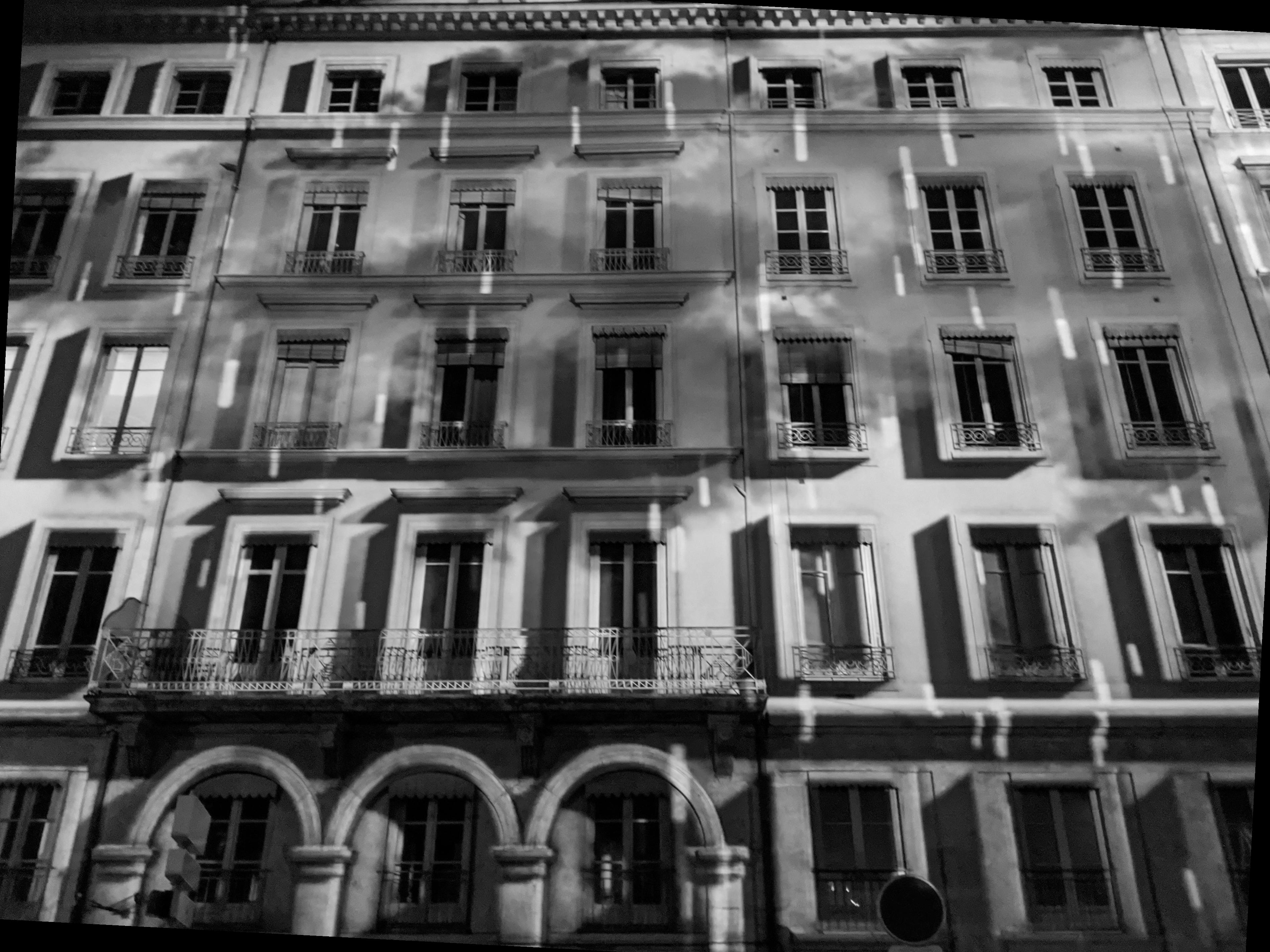
For part 1.3 we straightened images. Since in most images there is a preference for vertical and horizontal edges due to gravity, we were able to take different rotation angles of our images and compute a histogram of the gradient angles in our image and choose the proposed rotation which had the highest count of vertical and horizontal angles. Below, the straightened images are shown in the order of original image, straightened image, and lastly the histogram of the angles in the image. The majority of the images were successful except for image number 3, the house with the slanted roof. Since the algorithm aligns based on horizontal and vertical edges, it tried to correct the roof of the slanted house, which in reality is actually just slanted.
Straightened images
Part 2.1: Image "Sharpening"
For part 2.1 we sharpened images by subtracting our image convolved with the gaussian filter (the blurred image in part 1.2) from our original image.
Sharpened images

original image
sharpened alpha=1.3

sharpened alpha=2.0
I also sharpened my boyfriend's LinkedIn picture.

original image
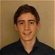
sharpened alpha=1.3
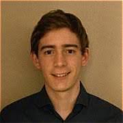
sharpened alpha=2.0
original image

sharpened alpha=1.3
sharpened alpha=2.0
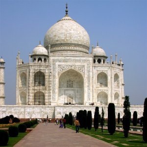
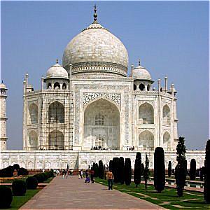
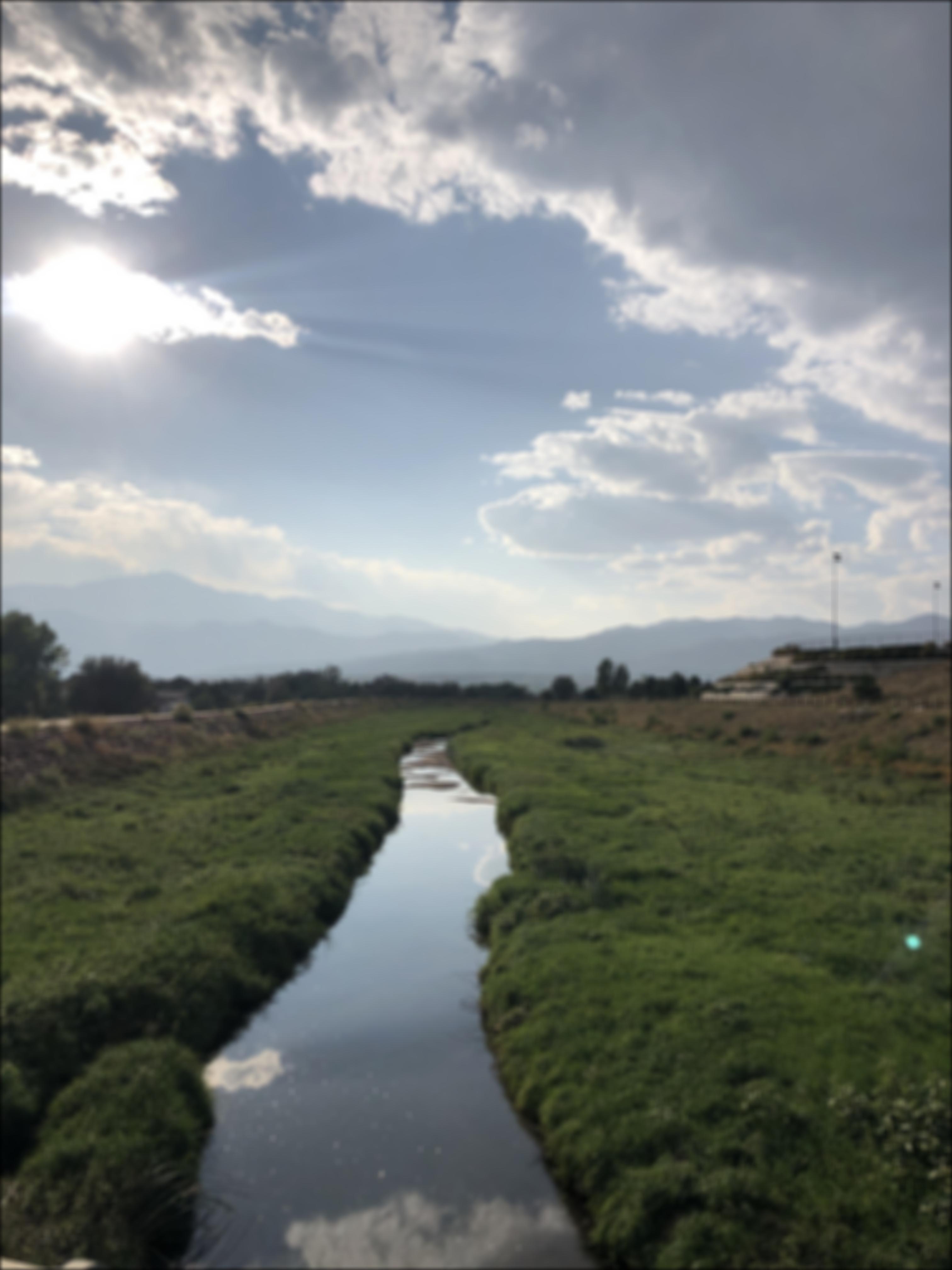
I took my photo of a river in colorado, unsharpened it using a gaussian filter, and then resharpened it with my unsharp mask. I noticed that the sharp image is different than the original. This is probably because we are removing low frequencies, which the original image did contain.
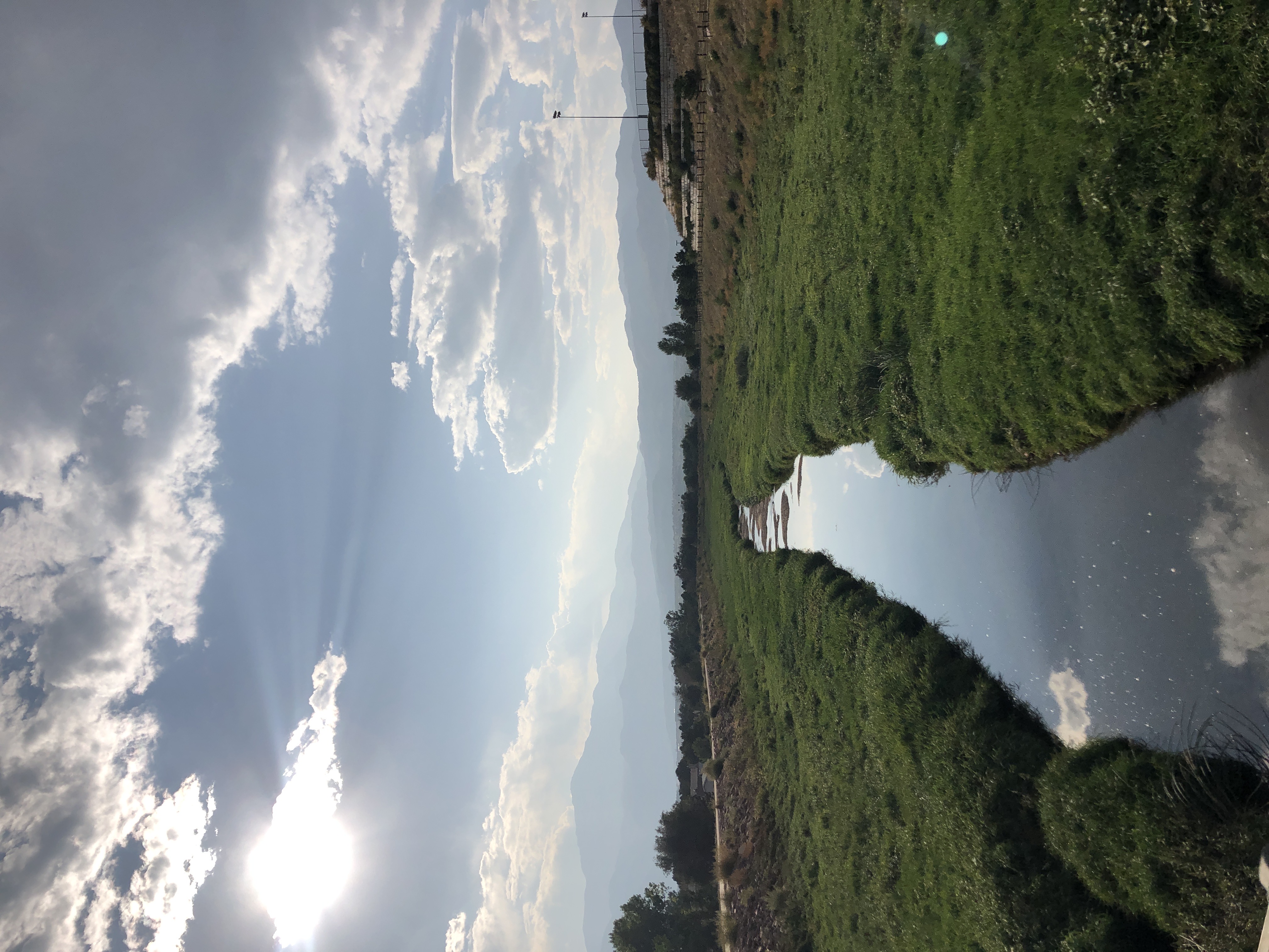
original image
unsharpened with gaussian(25,10)
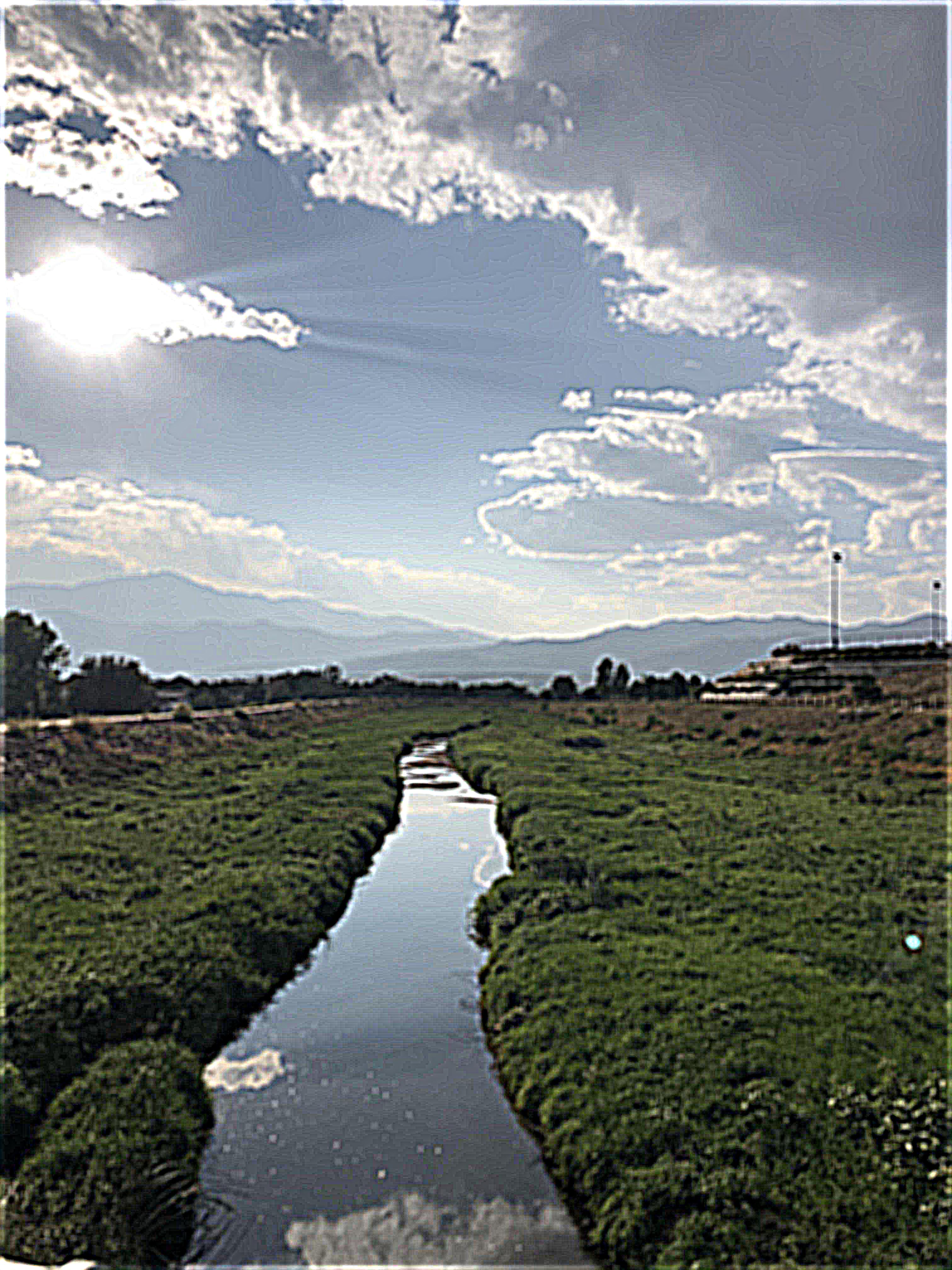
sharpened with gaussian(25,10)
Part 2.2: Hybrid Images
For part 2.2 we created hybrid images by choosing two images, aligning them, taking the high frequencies of one image, the low frequencies of the other image and combining them for the final image. For the low pass filter we use our classic gaussian, but for our high pass filter we use the laplacian of the gaussian filter or the unit impulse minus the gaussian filter.
A Hybrid Mr. Darcy: The stuff of Jane Austen's nightmares
My first hybrid image is a combination of the famous character Mr. Darcy from Jane Austen's Pride and Prejudice. I took Mr. Darcy from the P&P BBC Series played by Colin Firth and Mr. Darcy from the P&P movie starring Kiera Knightley played by Matthew Macfayden. Although Mr. Darcy is supposed to be both charming and handsome, the Mr. Darcy hybrid looks neither charming nor handsome, but instead quite scary.
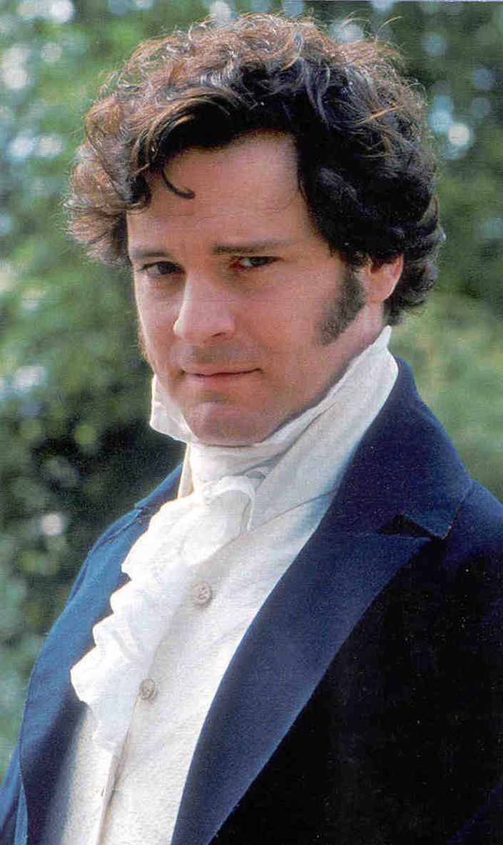
Image 1: Colin Firth
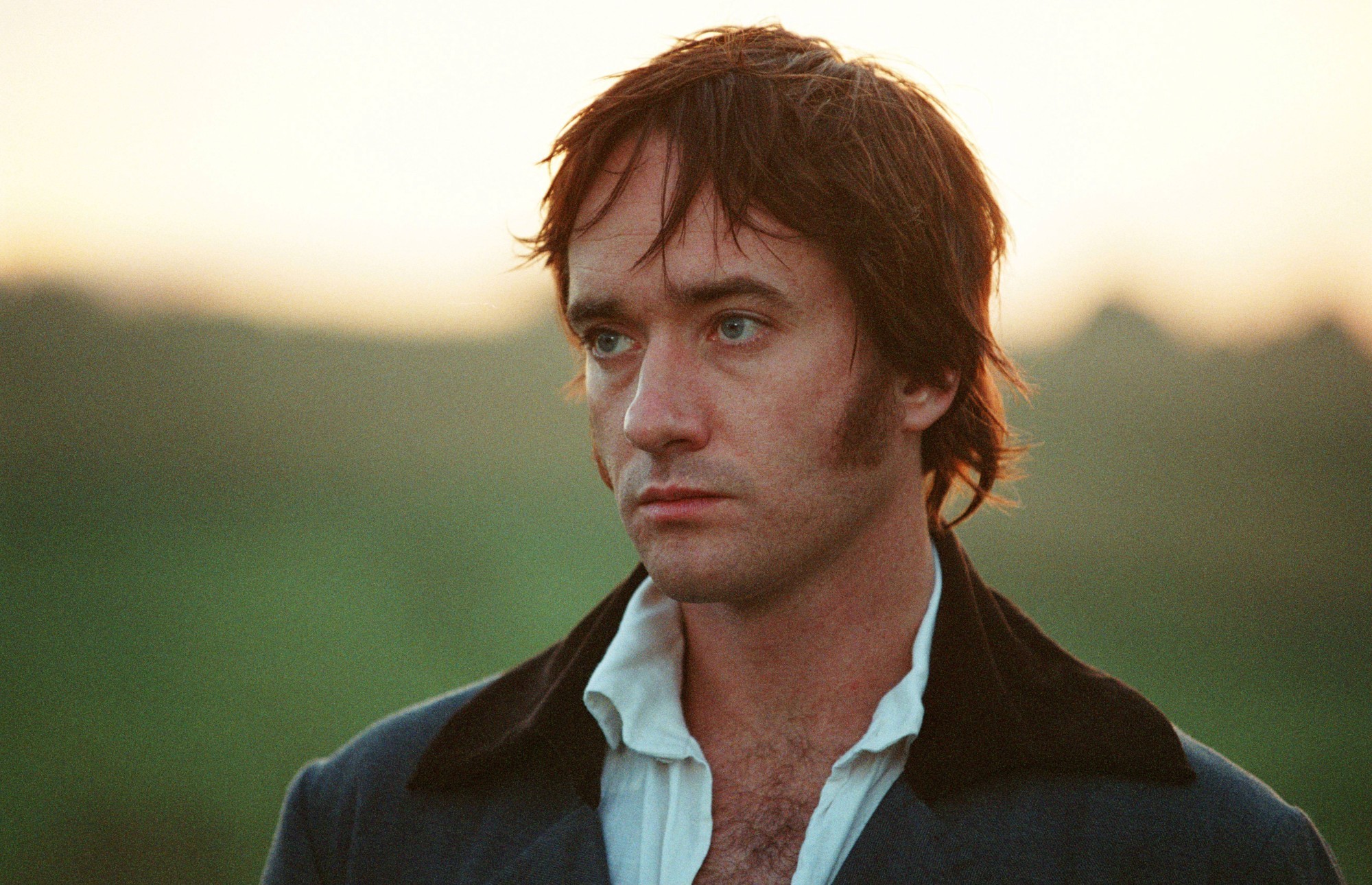
Image 2: Matthew Macfayden
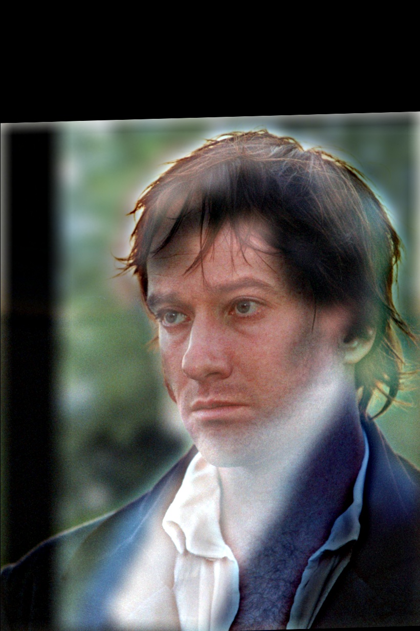
Mr. Darcy Hybrid
Hey all you cool cats and kittens!
During quarantine, the Netflix documentary Tiger King became one of the most popular shows in the US. In this image I combine Tiger King's Carole Baskin with a cat. Carole Baskin is the villian of Tiger King and known for being completely obsessed with cats. Watch her today on Dancing with the Stars!
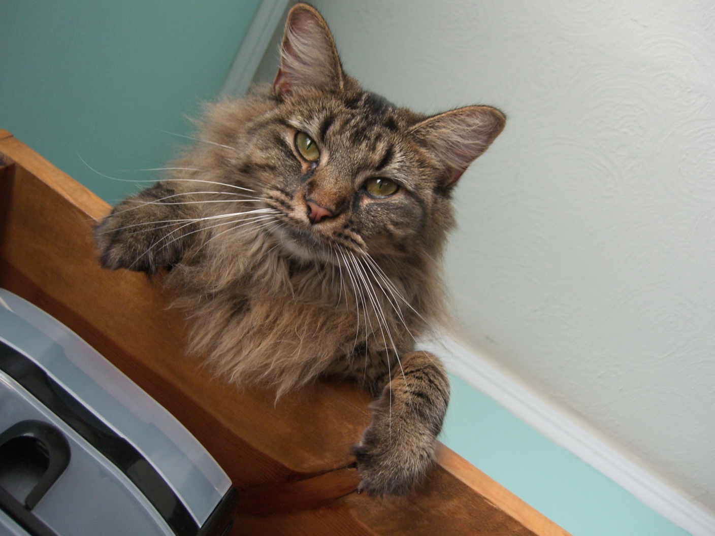
Image 1: Nutmeg
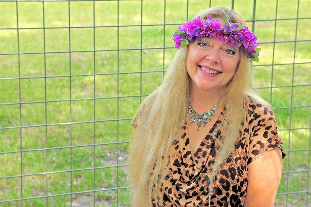
Image 2: Carole Baskin
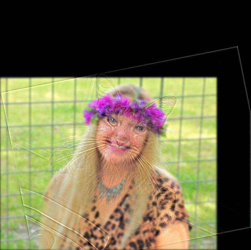
Carole-Cat Hybrid
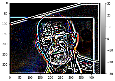
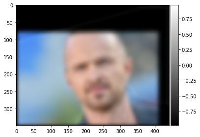
My favorite: Walter Pinkman or Jessie White?
One of my favorite shows of all time is Breaking Bad, so I decided to combine the faces of the two main characters Walter White and Jessie Pinkman. I think that this image looks the best, because the two original images looked very similar down to the characters' facial hair.
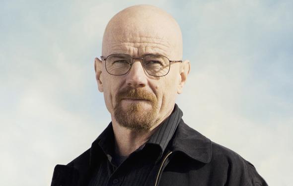
Image 1: Walter White
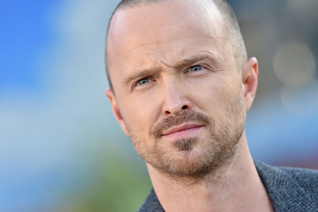
Image 2: Jessie Pinkman
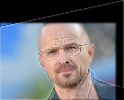
Walt-Jessie Hybrid
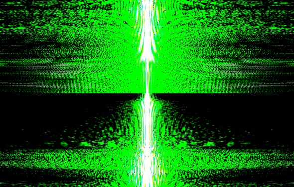
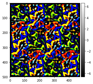
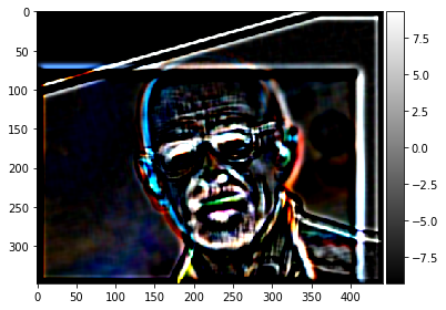
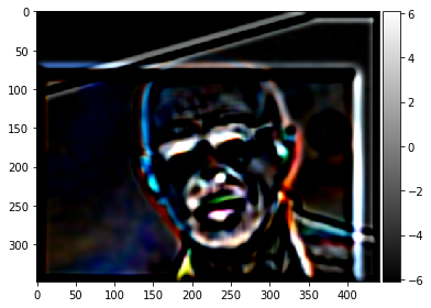
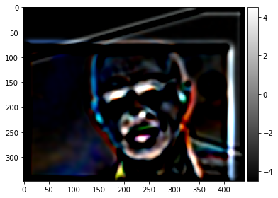
Fourier Walt
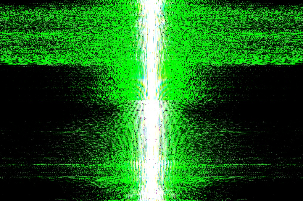
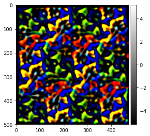
Fourier Jessie
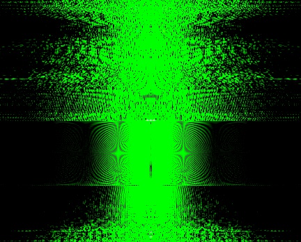
Fourier Filter Walt
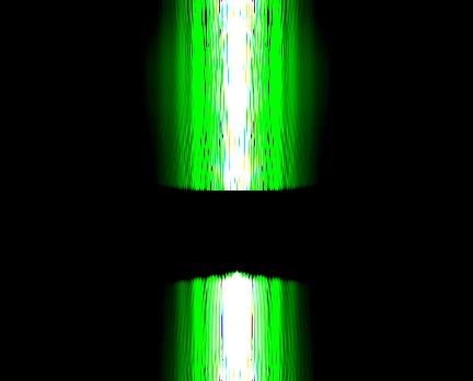
Fourier Filter Jessie
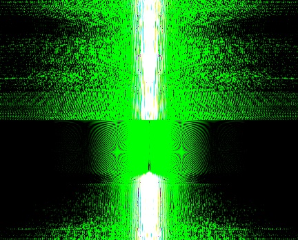
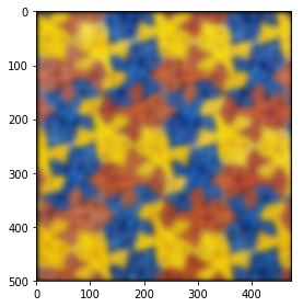
Fourier Filter Hybrid
Failure Case: Tina is not a unicorn :(
In this hybrid, I tried to combine Tina Belcher from Bob's Burgers with a unicorn, since unicorns and horses are her favorite animal. Because the images are very misaligned (the sizes are different, the features don't match up, the backgrounds are different) the images fail to align. Sorry Tina!
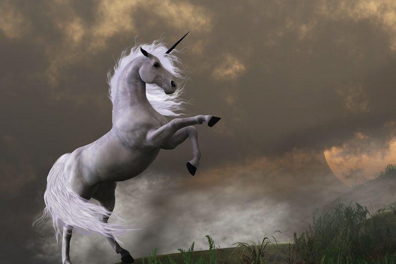
Image 1: Unicorn
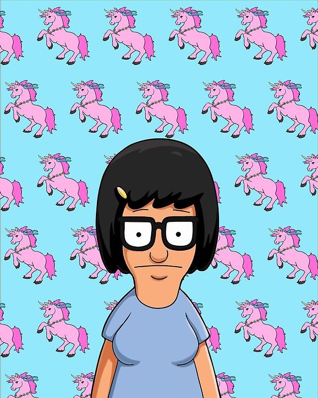
Image 2: Tina Belcher
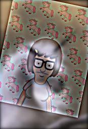
Tina-Unicorn Hybrid
Part 2.3: Gaussian and Laplacian Stacks
For part 2.3 we created Gaussian and Laplacian Stacks for images. This was done by repeatedly convolving an image with a gaussian filter for the gaussian stack and subtracting the differences between the gaussian stack to get the laplacian stack. The laplacian stack has the next level of the gaussian added to the end to make computation easier in the next part of the project.
Gaussian Stack: Fish(No. 55) M.C. Escher
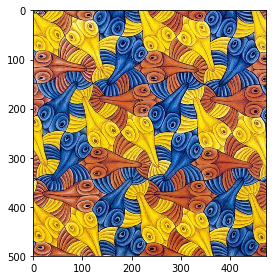
original image: level 0
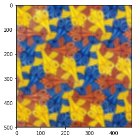
level 1

level 2
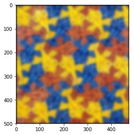
level 3

level 4
Laplacian Stack w/ Added Gaussian: Fish(No. 55) M.C. Escher
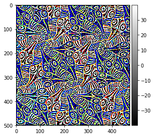
level 0
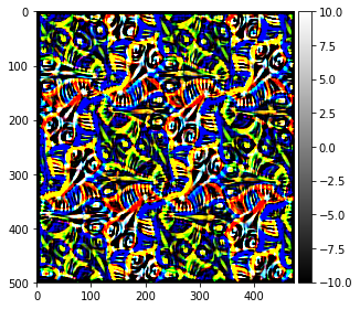
level 1
level 2
level 3
level 4 of the gaussian stack
Gaussian Stack: Walt-Jessie Hybrid

original image: level 0

level 1

level 2

level 3

level 4
Laplacian Stack w/ Added Gaussian: Walt-Jessie Hybrid
level 0
level 1
level 2
level 3
level 4 of the gaussian stack
Part 2.4: Multiresolution Blending
For part 2.4 we created blended images by alpha blending two images by combining their respective laplacian stack along with the last gaussian (as described in part 2.3) and applying a gaussian mask. See the Burt Adelson paper for more details.

Image 1: orange

Image 2: apple

Image 3: mask
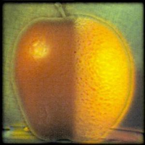
Image 4: orapple
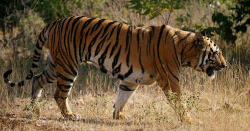
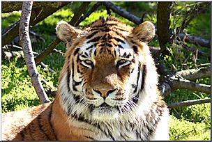
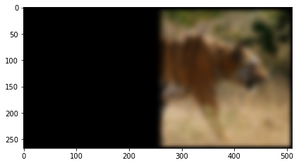
Image 1: tiger
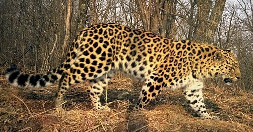
Image 2: leopard
Image 3: mask
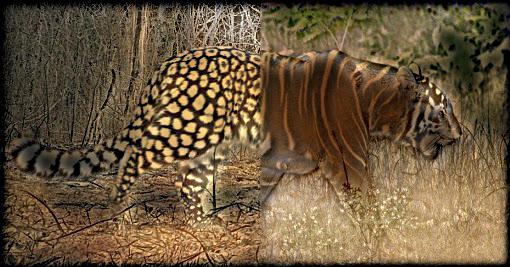
Image 4: leo-tiger
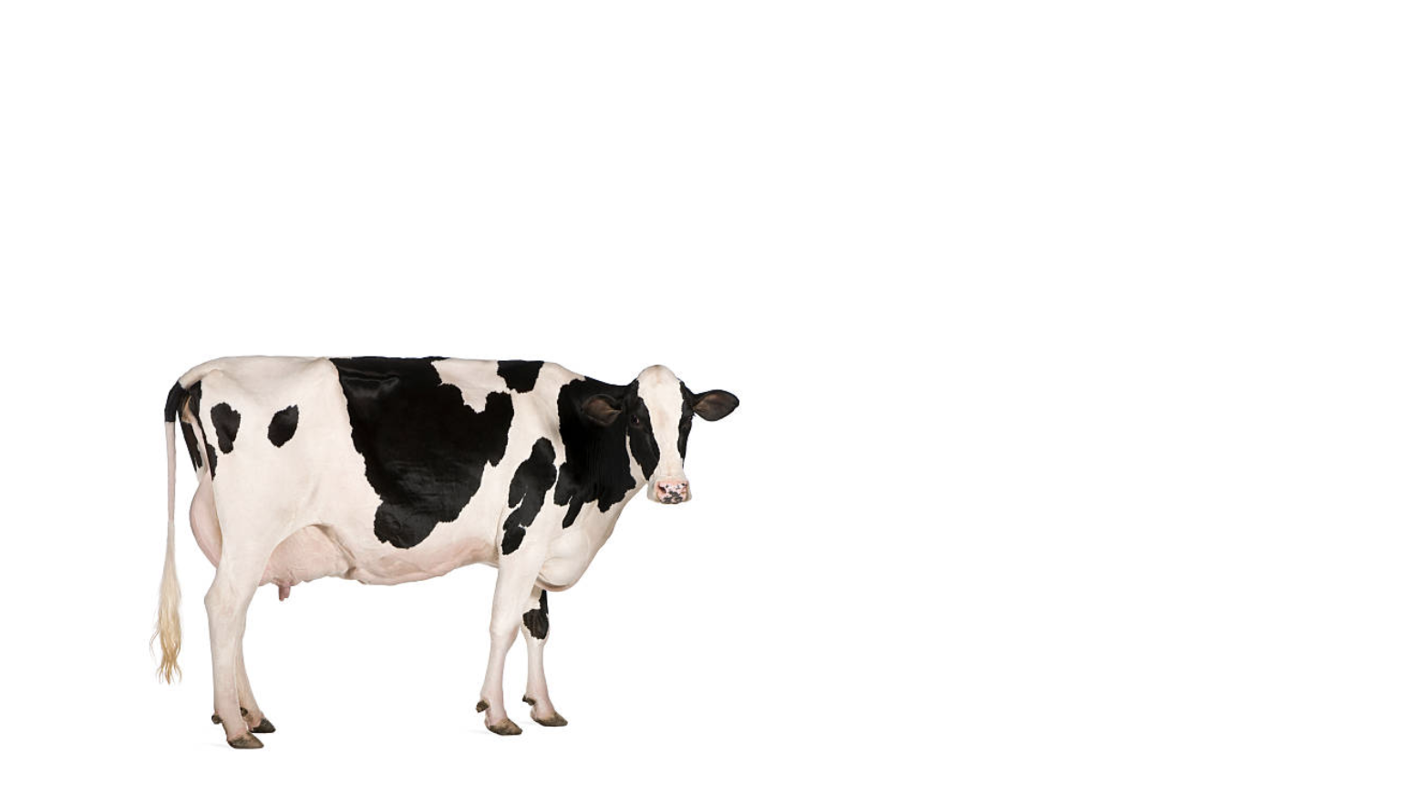
Image 1: cow
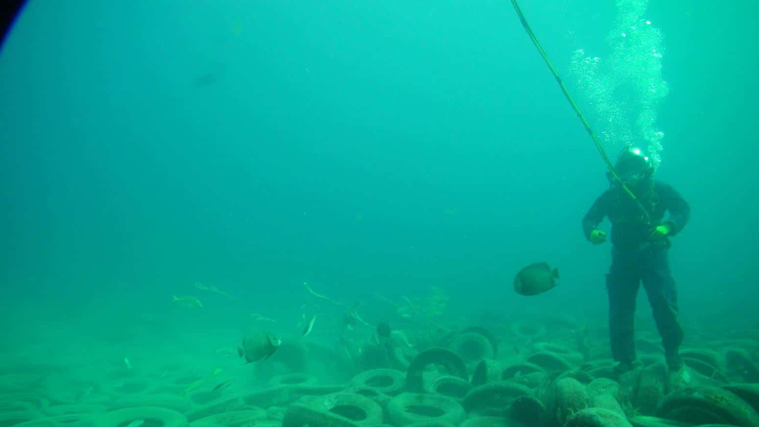
Image 2: ocean_floor
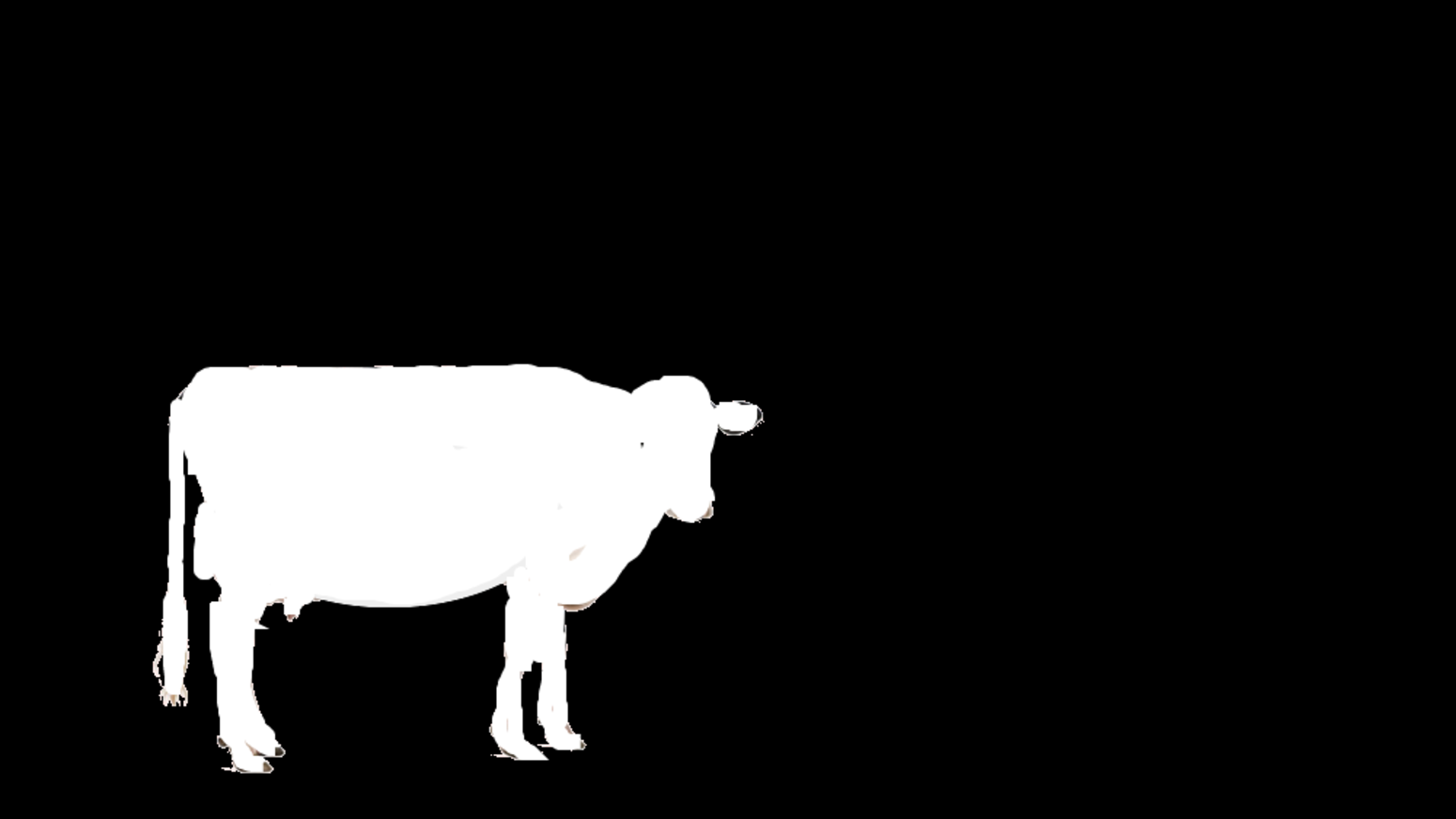
Image 3: mask
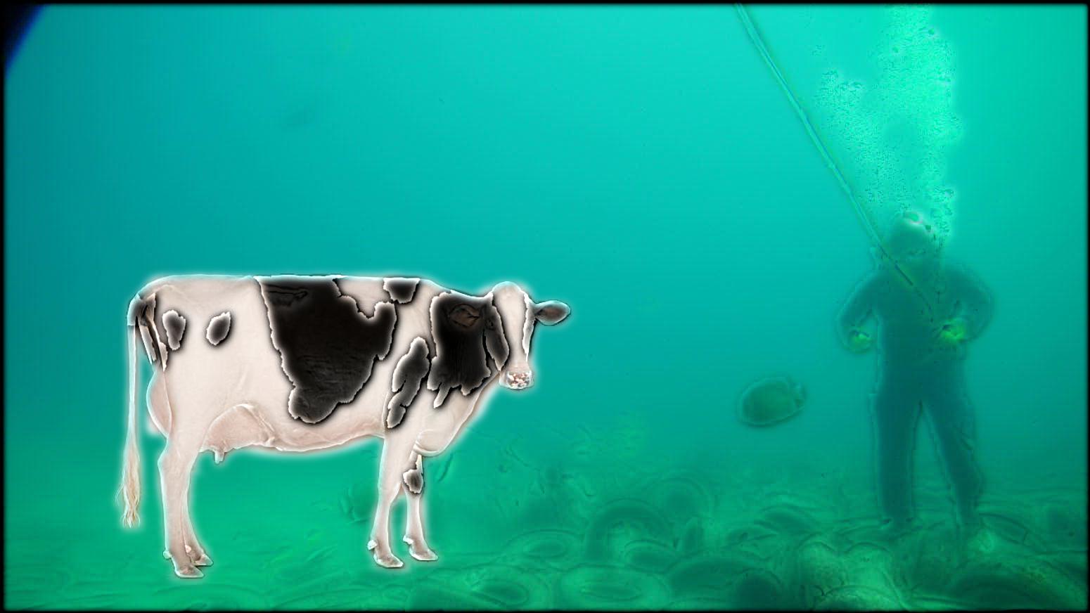
Image 4: underwater cow
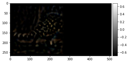
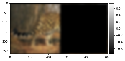
leopard stack
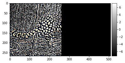
level 0
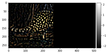
level 1
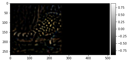
level 2
level 3
level 4 of the gaussian stack
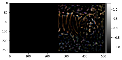
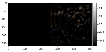
tiger stack

level 0
level 1

level 2
level 3
level 4 of the gaussian stack
Final Takeaways
I really enjoyed this project, as it was really fun to play with the images. My biggest takeaway probably had to do with the high pass/low pass filters. I understand what removing/adding high pass and low pass filters can do and also how the laplacian pyramid can be collapsed to create the original image.