
|
|

|
|
|
|
|
This assignment includes a lot of applications of filters and frequencies. We created filters and implemented functions to manipulate images for various usages such as image straightening, sharpening, blending, etc.
|
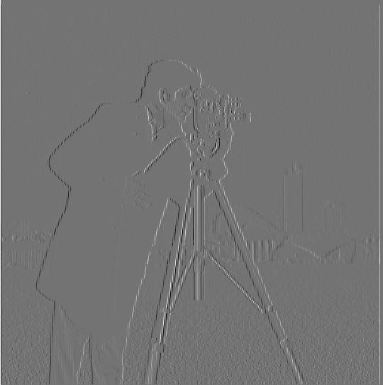
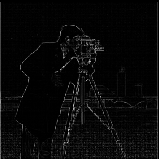
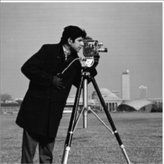
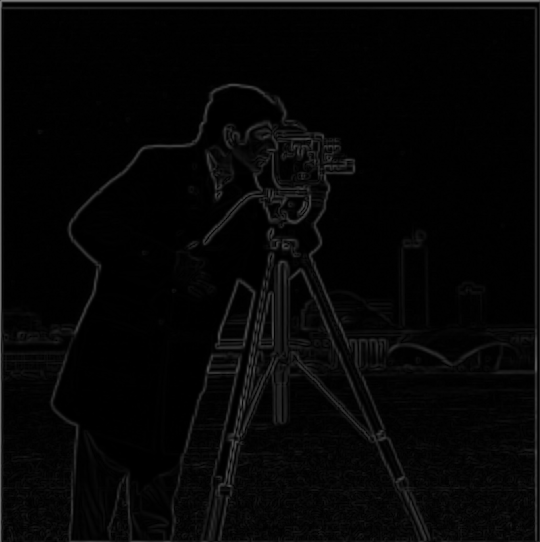
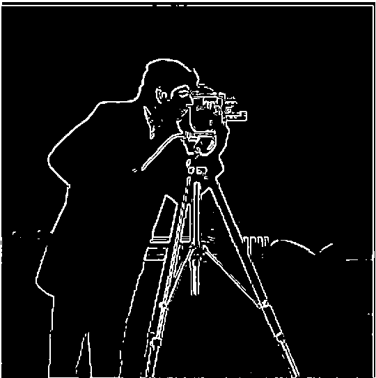
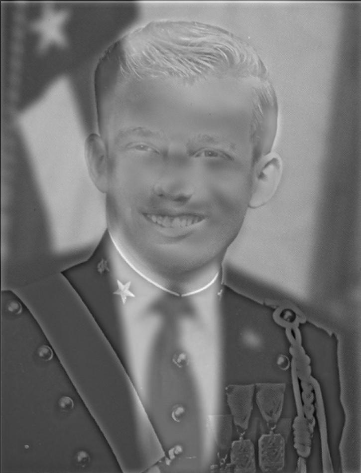
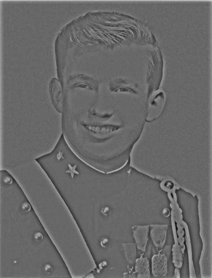
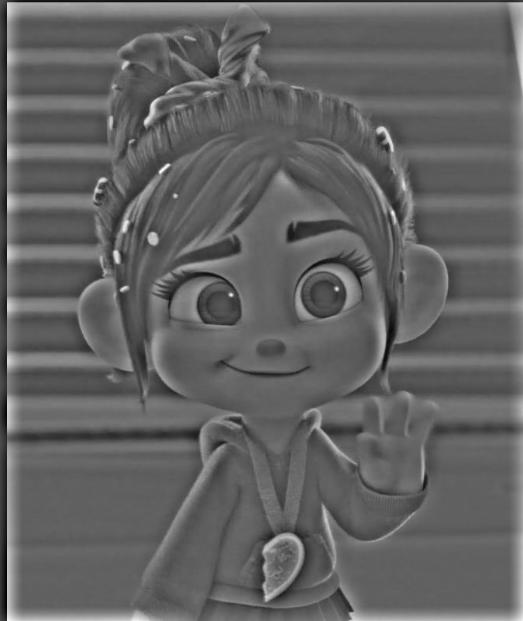
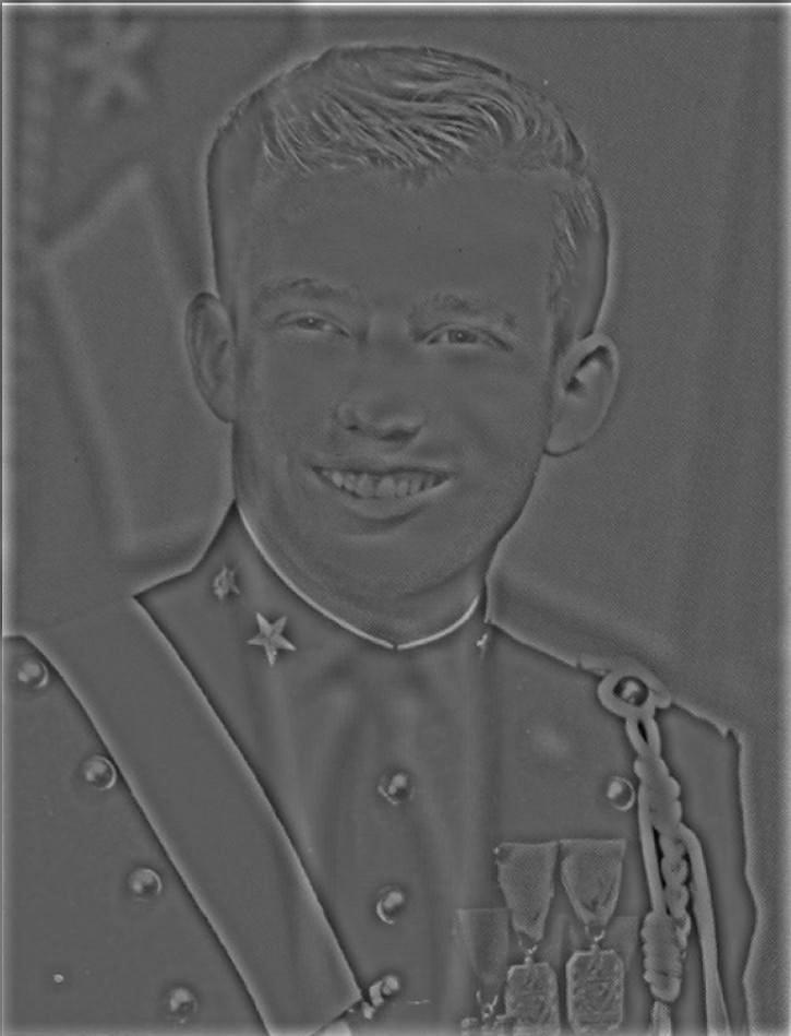
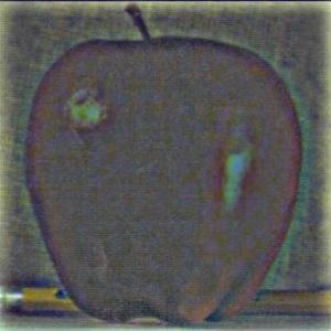
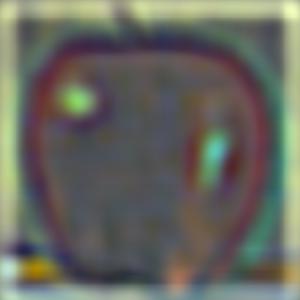
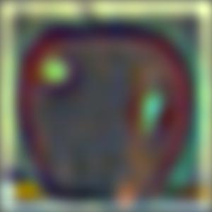
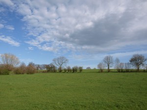
Firstly, we convolve the image with the finite difference operators dx and dy to get the partial derivatives of the image, then apply the Pythagoras's theorem to computer the gradient magnitude of the image. And I also binarize the result to with a certain threshold so that the edges are more obvious.
dx |
dy |
gradient magnitude |
binarized edge image |
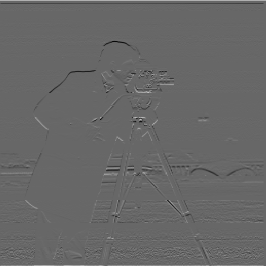
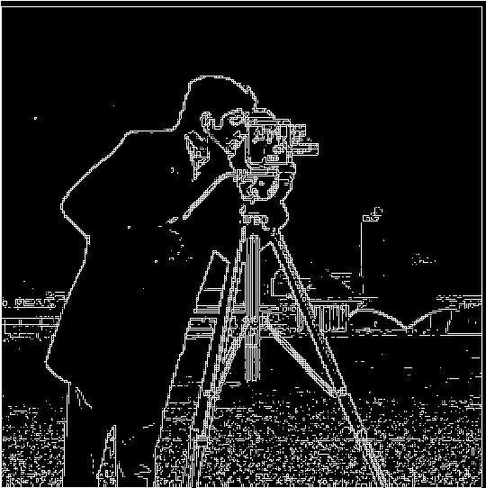
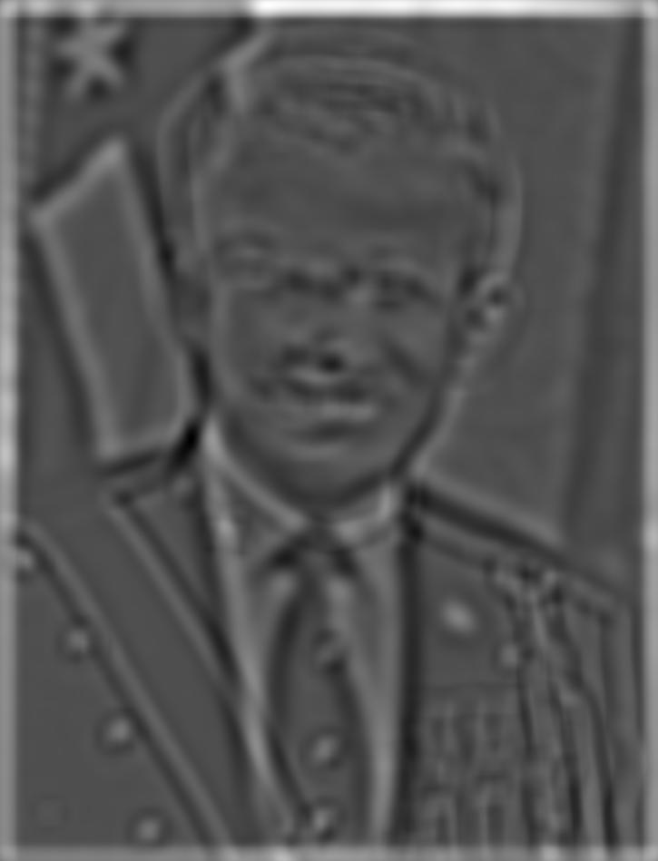
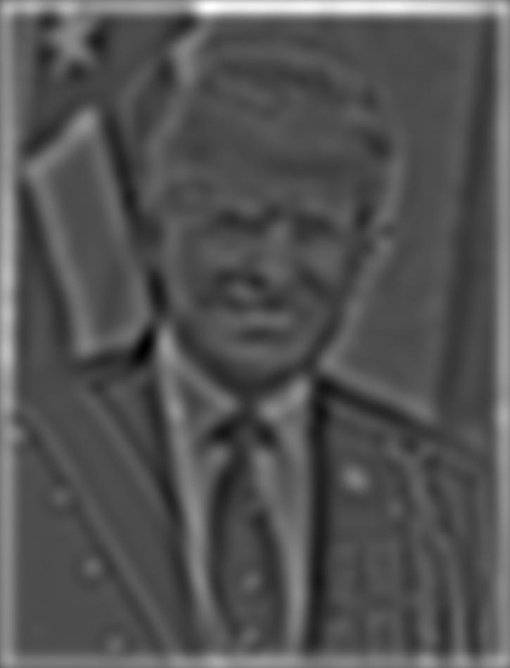
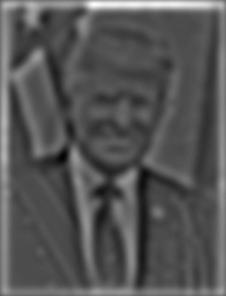
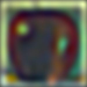
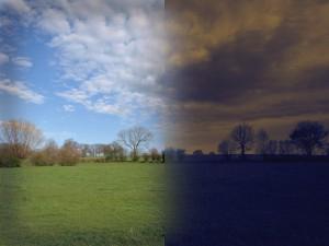
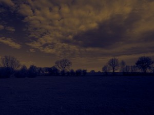
As we can see above, the binarized edge image is still quite noisy. To improve our result, I convolve the image with the Gaussian filter to blur the image before computing the gradient. With the same procedure afterwards, the resulting binarized edge image is now much cleaner and represents all the true edges in the original image more accurately.
|
original |
blurred |
gradient |
binary edge |
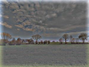
The above algorithm requires us to do two convolutions with the image. In fact, we can reduce it to a single convolution if we compute the derivative of gaussian filters first and convolve the image with them instead of the finite difference operators. The result would be the same due to the associative property of convolution.

dx of gaussian filter |

dy of gaussian filter |

1 convolution with image |
2 convolutions with image |
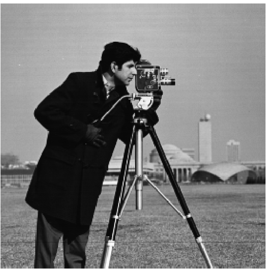
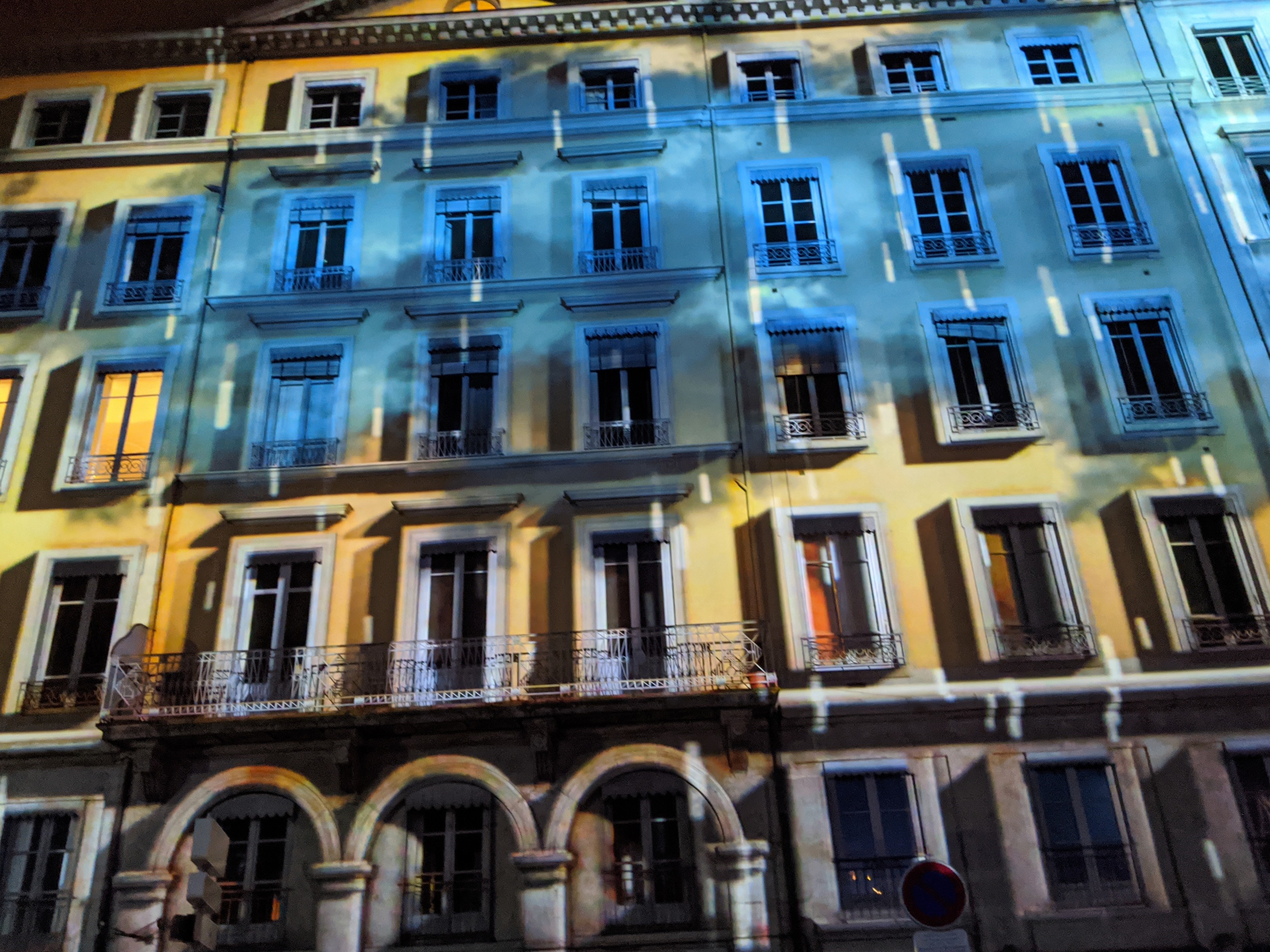
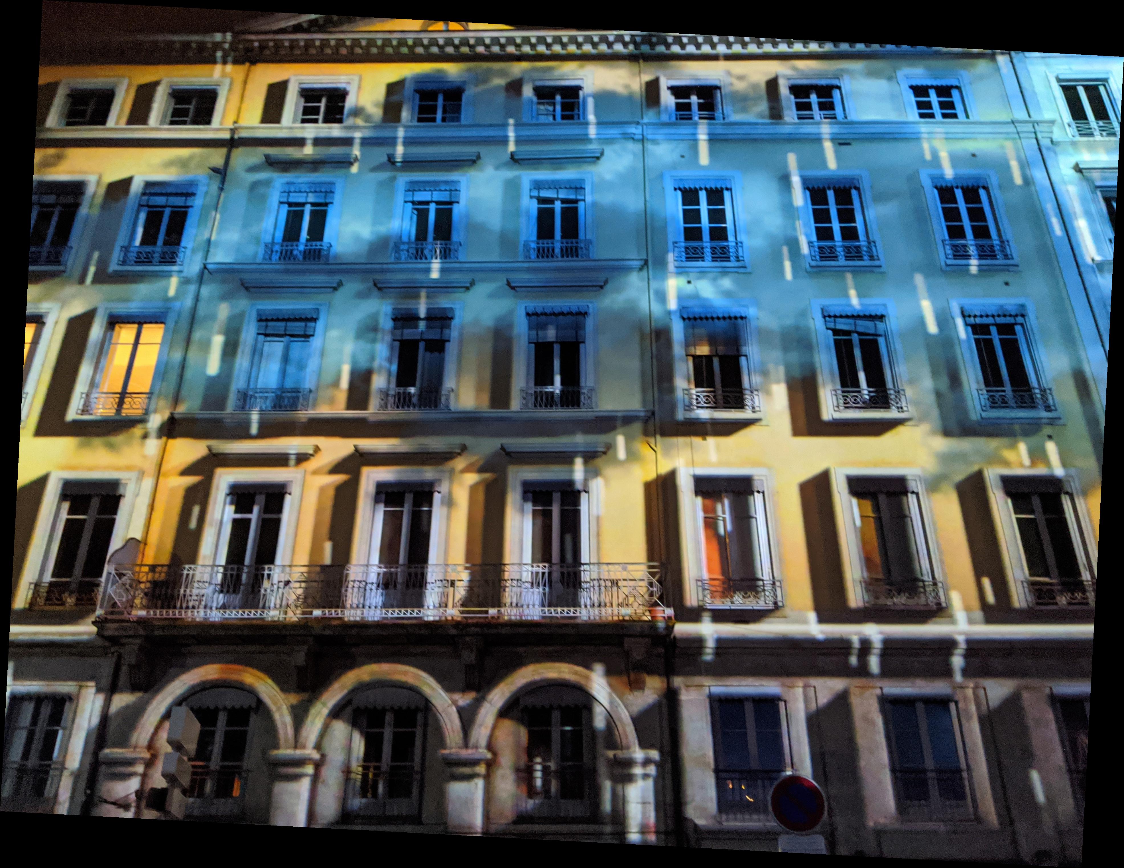
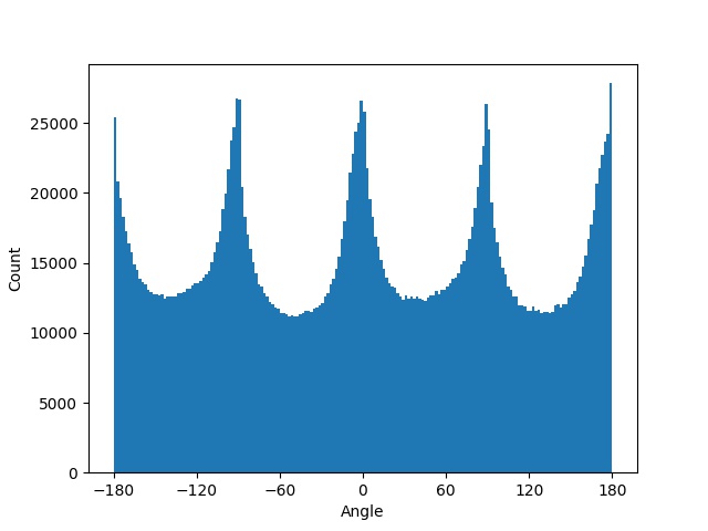
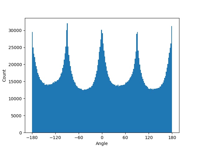
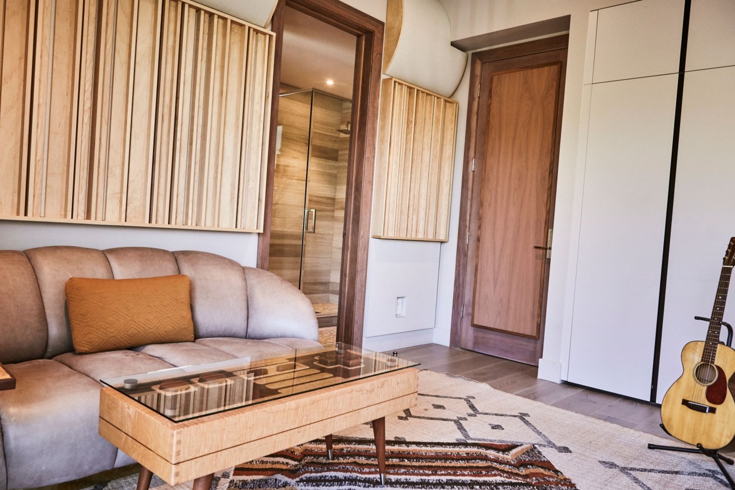
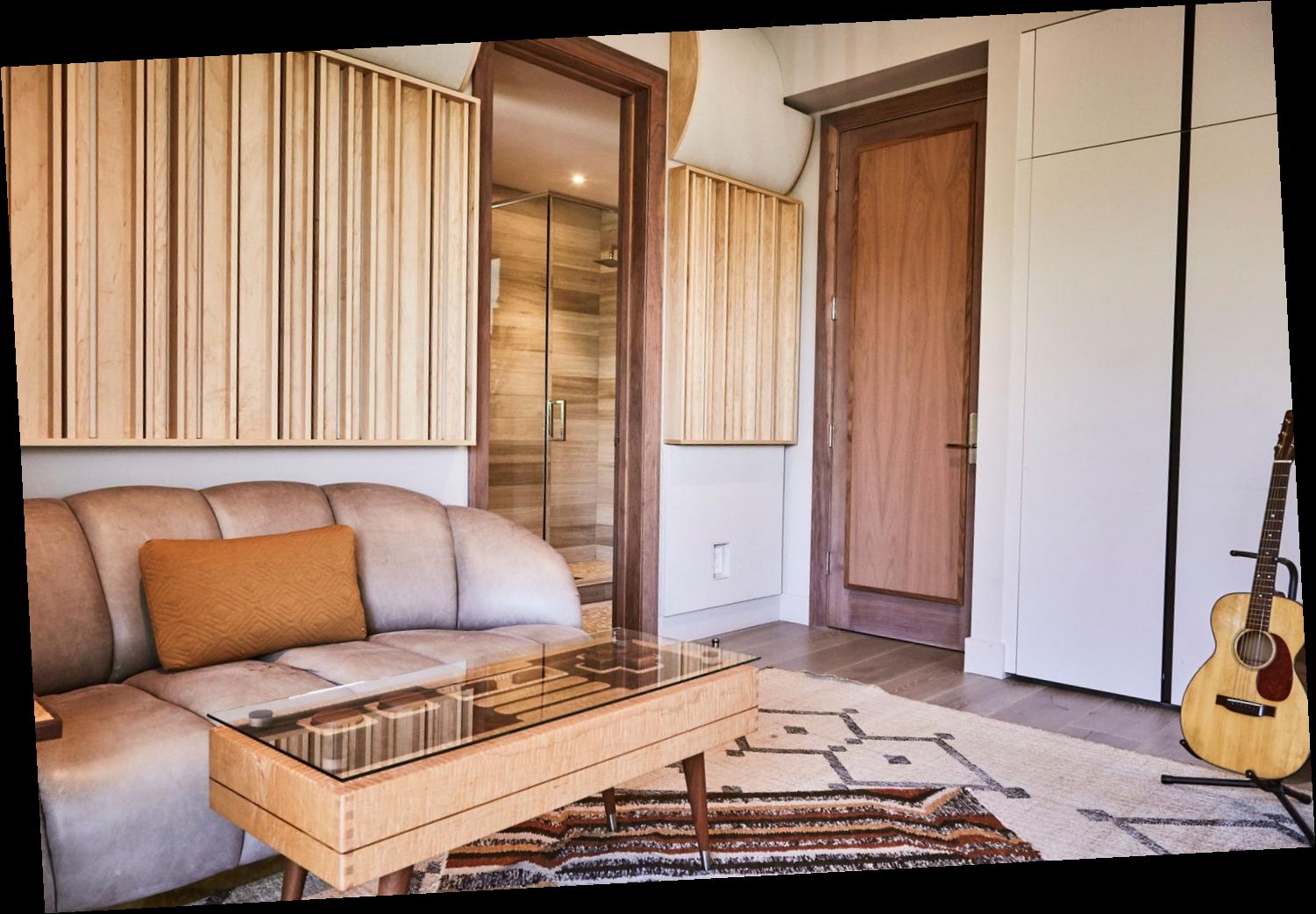
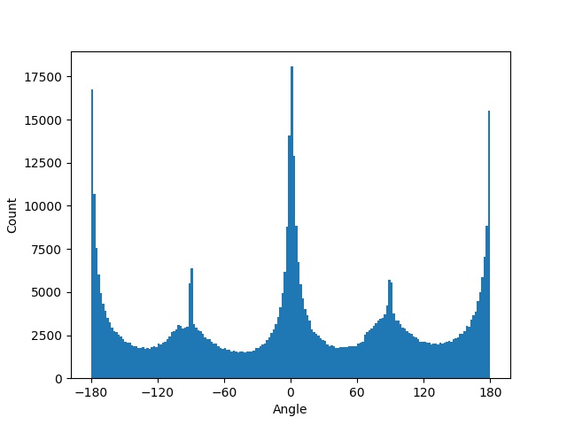
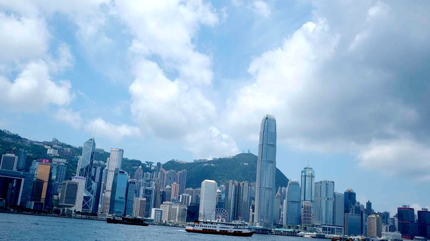
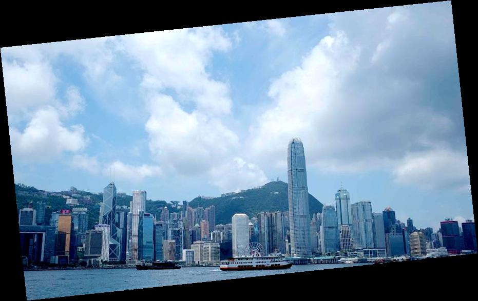
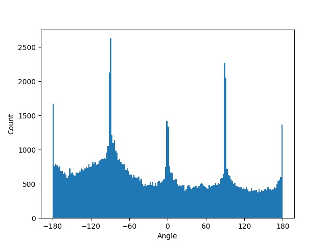
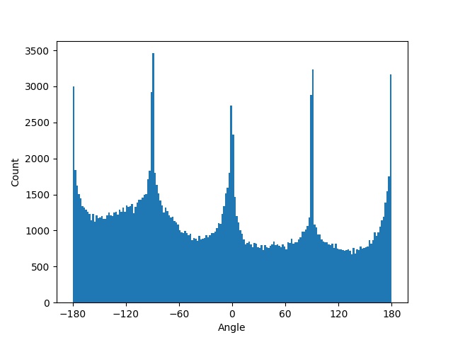
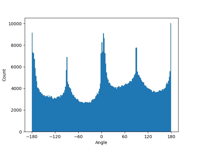
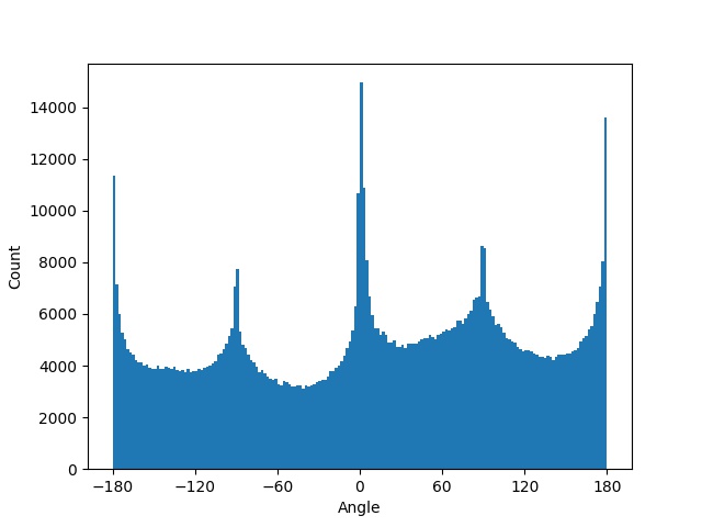
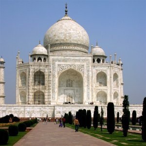
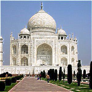
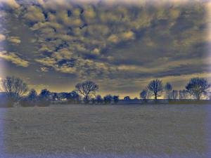
In this section, I implemented an algorithm to automate the image straightening process by detecting the number of vertical and horizontal edges within a range of angles and return the one with the most vertical and horizontal edges. Here are a few examples along with their histograms counting their number of edges in each angle. The algorithm maximizes the ones that are around 180°, 90°, 0°, -90°, or -180°.
|
|
|
|
|
|

|
|
|
|
|
|
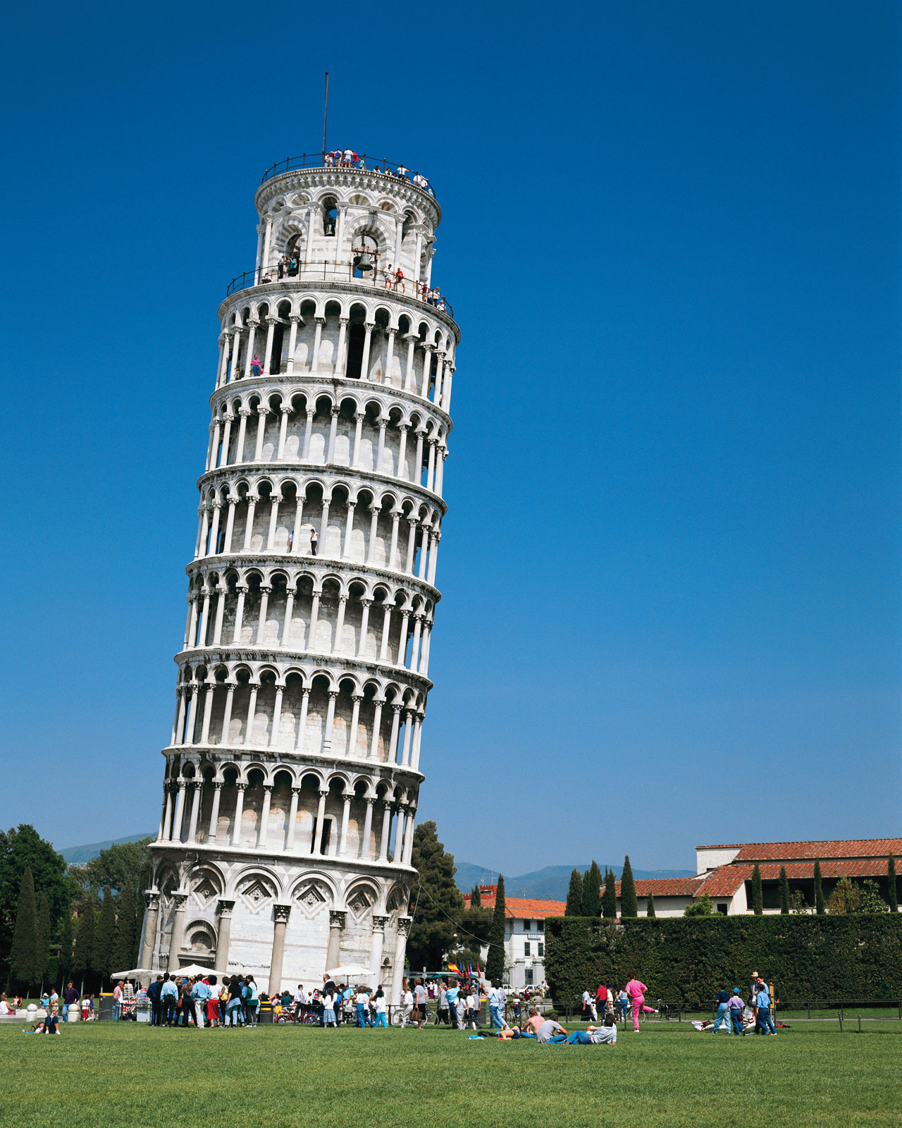
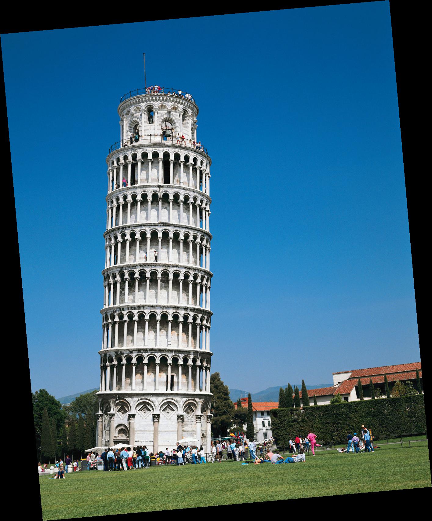
Here is a failure case where my program attempted to "straighten" the Tower of Pisa because there is a preference for vertical and horizontal edges:
|
|
|
|
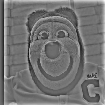
"Sharpening" an image basically means adding more high frequencies to it. We can obtain the "high frequencies" by subtracting the original image by its blurred version. Adding these "high frequencies" back to the original image achieves the sharpening affect.
original |

blurred |
sharpened |
original |

blurred |
sharpened |
Hybrid images are made by blending the high frequencies of one image with the low-frequencies' portion of another. High frequency dominates at close distances while not visible from far away. Therefore, we can see two different images at different distances.

|
|
|

|
|
|
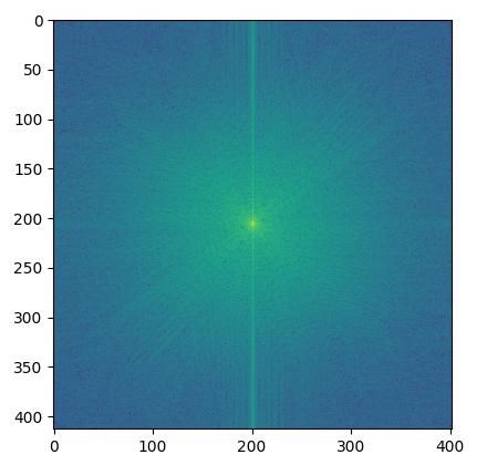
FFT of pooh.jpg |
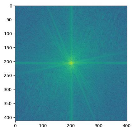
FFT of xi.jpg |
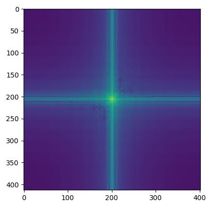
FFT of low pass pooh.jpg |
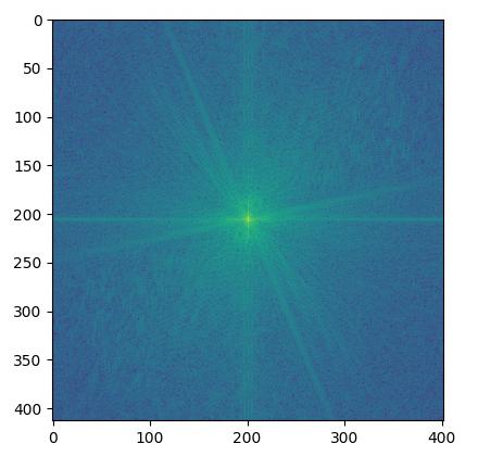
FFT of hybrid image |
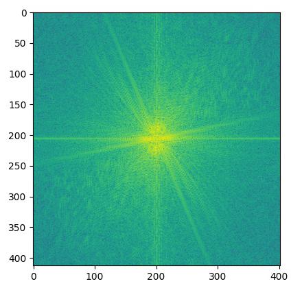
FFT of high pass xi.jpg |
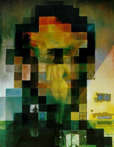
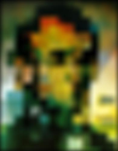
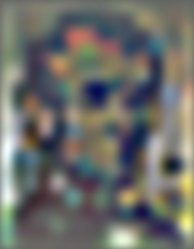
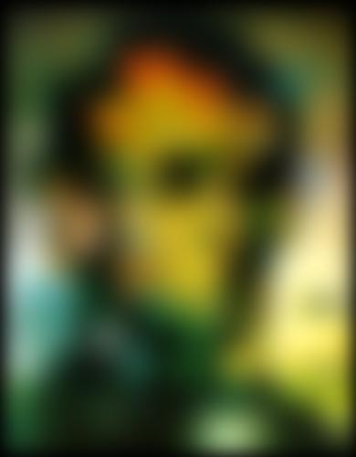
If we try to blend two images with very different shapes, the resulting hybrid image might look unnatural:

|

|
|
|
|
|
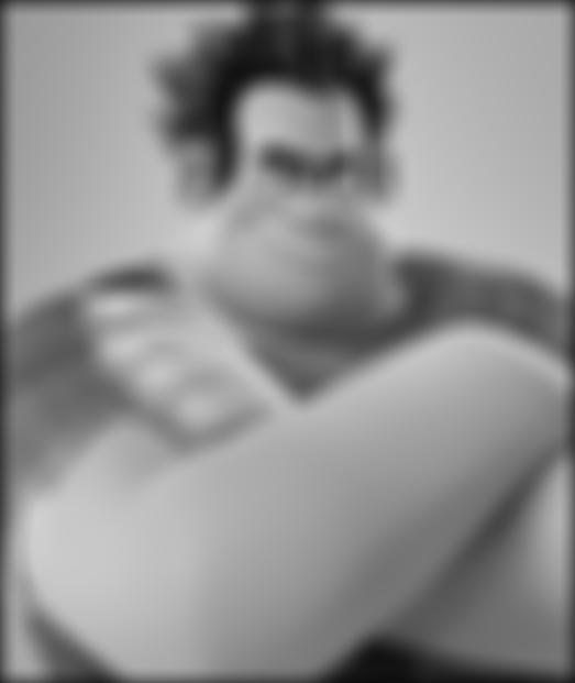
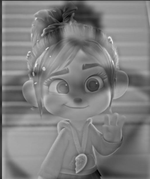
In the part, I implemented the Gaussian and Laplacian stacks which will be used for multi-resolution blending in the next part.
|
|
|

|
|

|
|
|
|

|
|
|

|
|

|

|
|

|
|
|
|

|
|

|
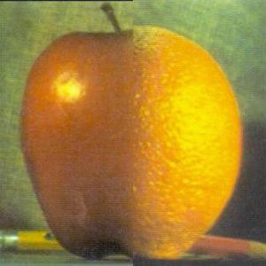
We can join two images smoothly by using multi resolution blending. In this part, I implemented the method described in this paper and here are the results:
|
|
|
|
|
|
|
|
|
|
|
|
|
|
|
|

|

|

|

|

|

|
|
|
|
|
|
|
|
|
|
|
|
|

|

|
|

|

|

|

|

|

|