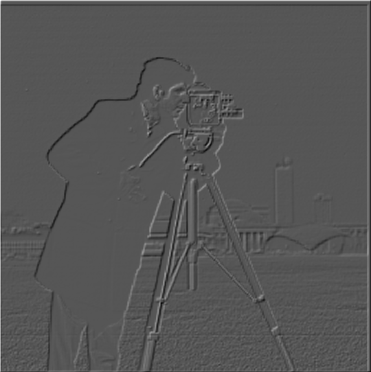
— dx |
— dy |
— dxy |
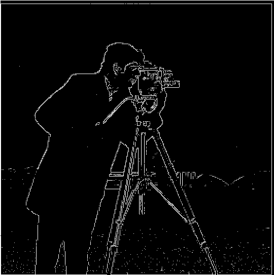
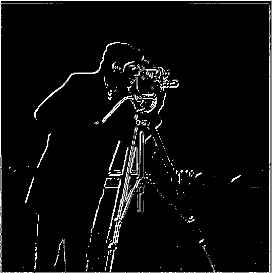
— threshold: 0.0010 |
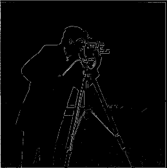
— threshold: 0.0015 |

— threshold: 0.0020 |
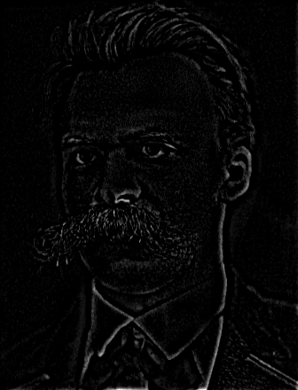
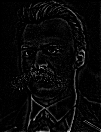
Images are data. They can be interpreted to become information. Interpretation requires Difference (a distinction, a detail, something that stands out). Visually, Difference can take on many qualities: color, texture, consistency. To be employed in Computer Vision, though, it must be somehow quantified. Hence enters the concept of change, and the mathematical study of change, differential calculus.
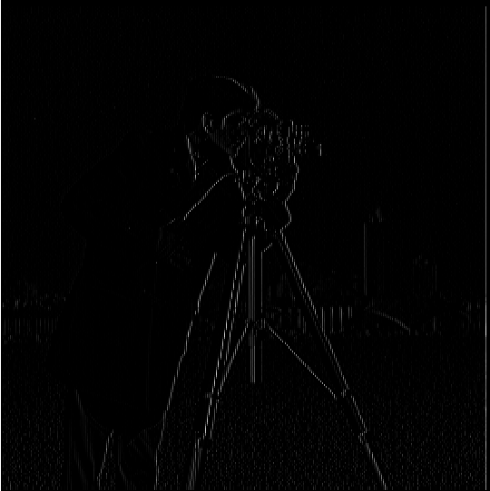
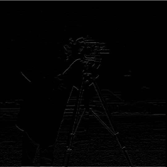
The edges of an image—its contours, those elements which delineate forms, and ultimately, make the symbols that provide us with meaning—are primarily a sharp change in color. In differential calculus, sharp changes are denoted by peaks in the gradient. Developing methods to accurately and efficiently compute the gradient of an image is, therefore, essential deriving or communicating meaning through vision.
That said, images, unlike other signals, are two-dimensonal, which signifies that computing their gradient is a bit more complicated than taking a derivative. Namely, the gradient (total derivative) must be computed as a function of the partial derivatives in each dimension. Now, on the (very, very) bright side, since images (at least within computer screens) are represented as discrete signals, no obscure calculus rules need to be memorized. The dot product says hi (and winks)!
Practically: the partial derivative of a line of pixels along a dimension (for example, the x- or y-axis) is the extent to which each of its constituent pixels is distinguishable from its neighbors along that line. The total derivative, therefore, is the extent to which every pixel in the image is different from its neighbors, along both dimensions.
Algorithm-wise, the image gradient can be implemented by first constructing two arrays of finite difference operators, one for each dimension. A finite difference operator is nothing more than a vector whose dot product with any other vector is the result of subtracting the elements of the other vector, in order. When convolved with an image, a finite difference operator yields the partial derivative of the image in the direction along its dimension. Joined together, two finite difference operators form a kernel. When convolved with the image, such kernel yields the gradient.
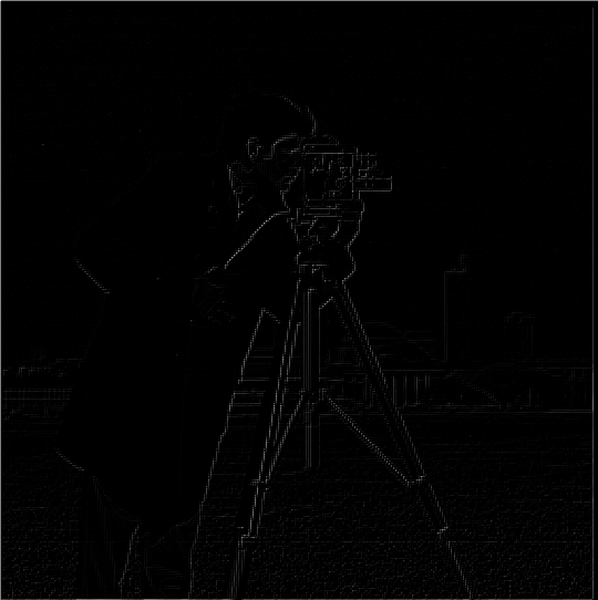
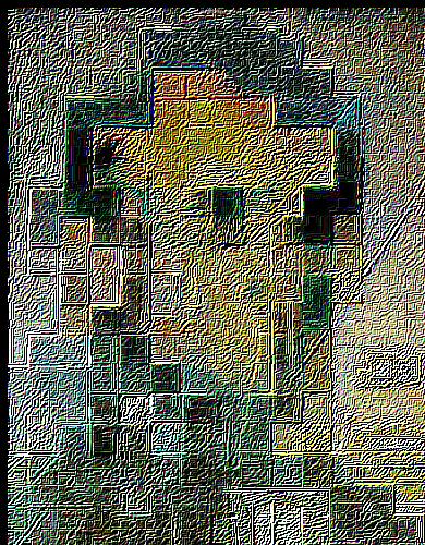
Having thus examined the role of the image gradient as morphogenic Difference, only one more concept needs to be introduced: the threshold. Thresholds are intensive points used to (subjectively?) separate, and therefore identify, that which is from that which is not. For example, the last three of following Cameraman pictures are the result of taking the image gradient, and applying a threshold. Any pixel intensity above the threshold is rounded up to 1 (is considered an edge). Any pixel intensity below the threshold is rounded down to 0 (is not considered an edge). Voilà.
|
— dx |
— dy |
— dxy |
|
— threshold: 0.0010 |
— threshold: 0.0015 |
— threshold: 0.0020 |
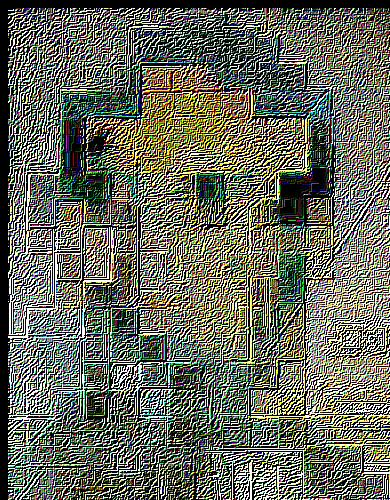
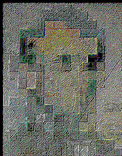
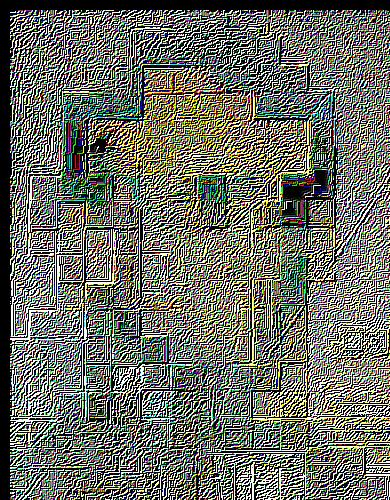
A shortcoming of taking the gradient of the image directly is that the latter, due to its sampled nature, is subject to noise. This results in detecting edges and artifacts that do not trully exist. Enter filtering. By selectively choosing which frequencies to keep from the image, the output will constitute (almost) only pertinent information.
The filter implemented for this project is known as Gaussian, as it involves a kernel made of a Gaussian (aka. Normal) distribution. The image in question is convolved with the kernel. As such, the intensity of the pixel in the middle of an area of the image having the size of the kernel, will become the weighted average of intensities in that area (with intensities closer to the center being assigned a higher weight).
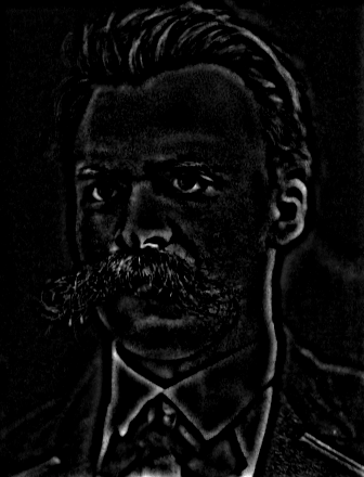
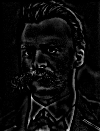
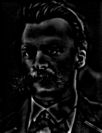
Notice the difference that filtering with a Gaussian before performing the gradient computationmakes. The following images of the Cameraman where first passed by a Gaussian filter with a kernel size of 3 and a standard deviation of 1.6. The image gradient, unlike in the previous part, now produces images that are gray rather than black and white. This occurs because a blurry image has less variation in frequency. Edges that used to be white are now a little darker. Parts that used to be black are now a little lighter. Everything is a bit more homogeneous.
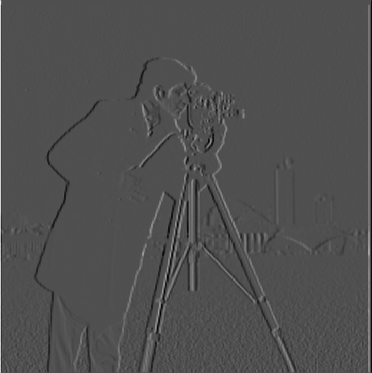
— dx |
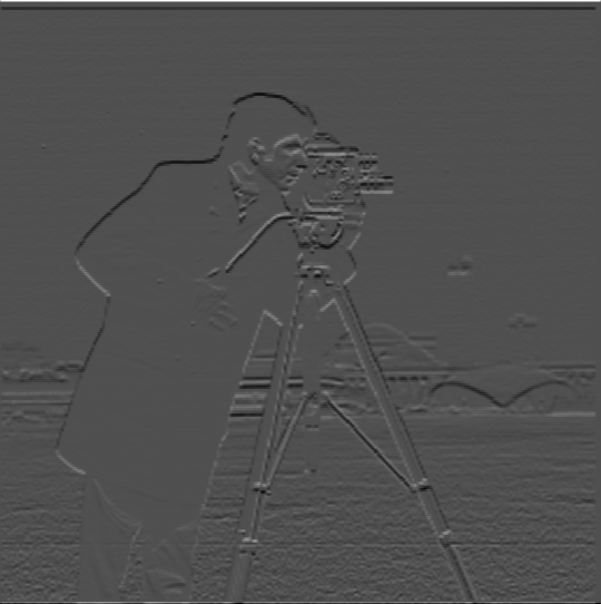
— dy |
— dxy |

— threshold: 0.0002 |
— threshold: 0.0005 |
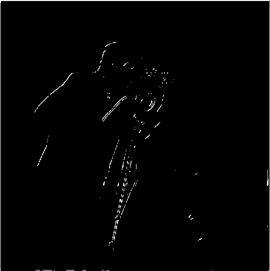
— threshold: 0.0010 |
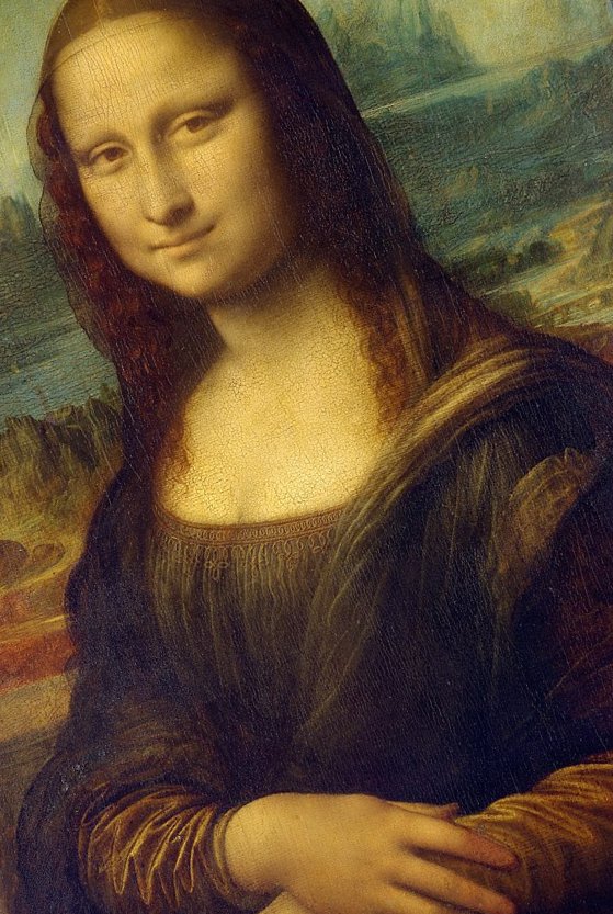
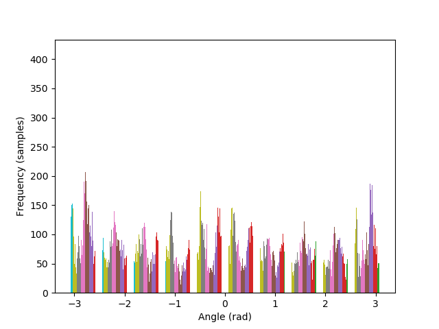
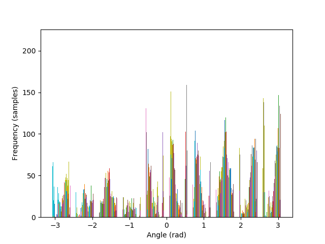
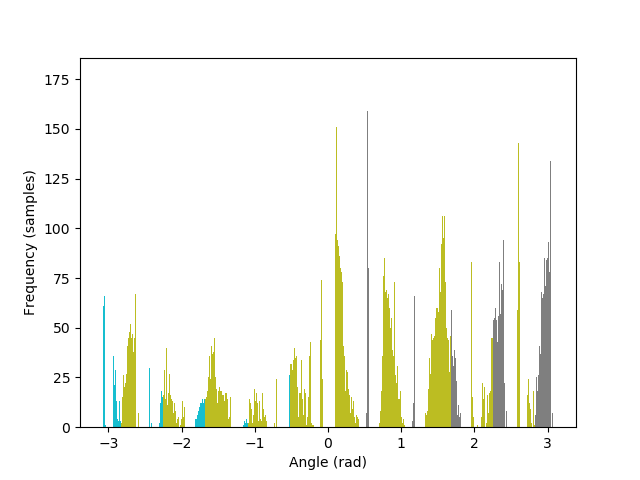
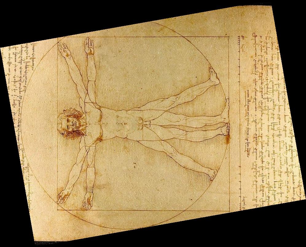
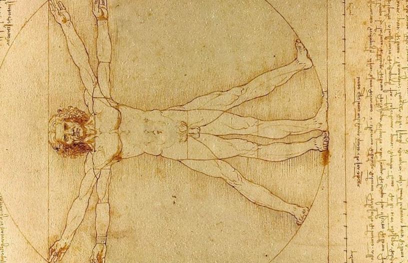
Images can be straightened programatically by testing their orientation along a set of rotations, and keeping the rotation that performs better in terms of maximizing the number of horizontal and vertical edges in the scene. The intuition behind such algorithm lies in the fact that, due to gravity, humans have a statistical preferences for lines parallel to, and orthogonal to, the ground.
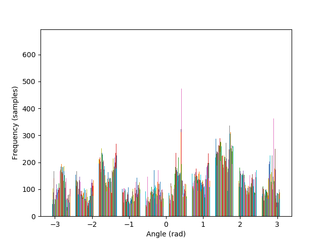
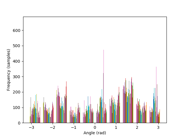
The metric to count horizontal and vertical edges is straightforward: first compute the gradient orientation at each pixel, which is simply the arctan of the ratio between the partial derivatives. Then, take the cos and sin of this orientation, and multiply them together. The more the gradient orientation approaches 0, 90, 180, or 270 degrees, the closer it will be to zero, and vice versa.
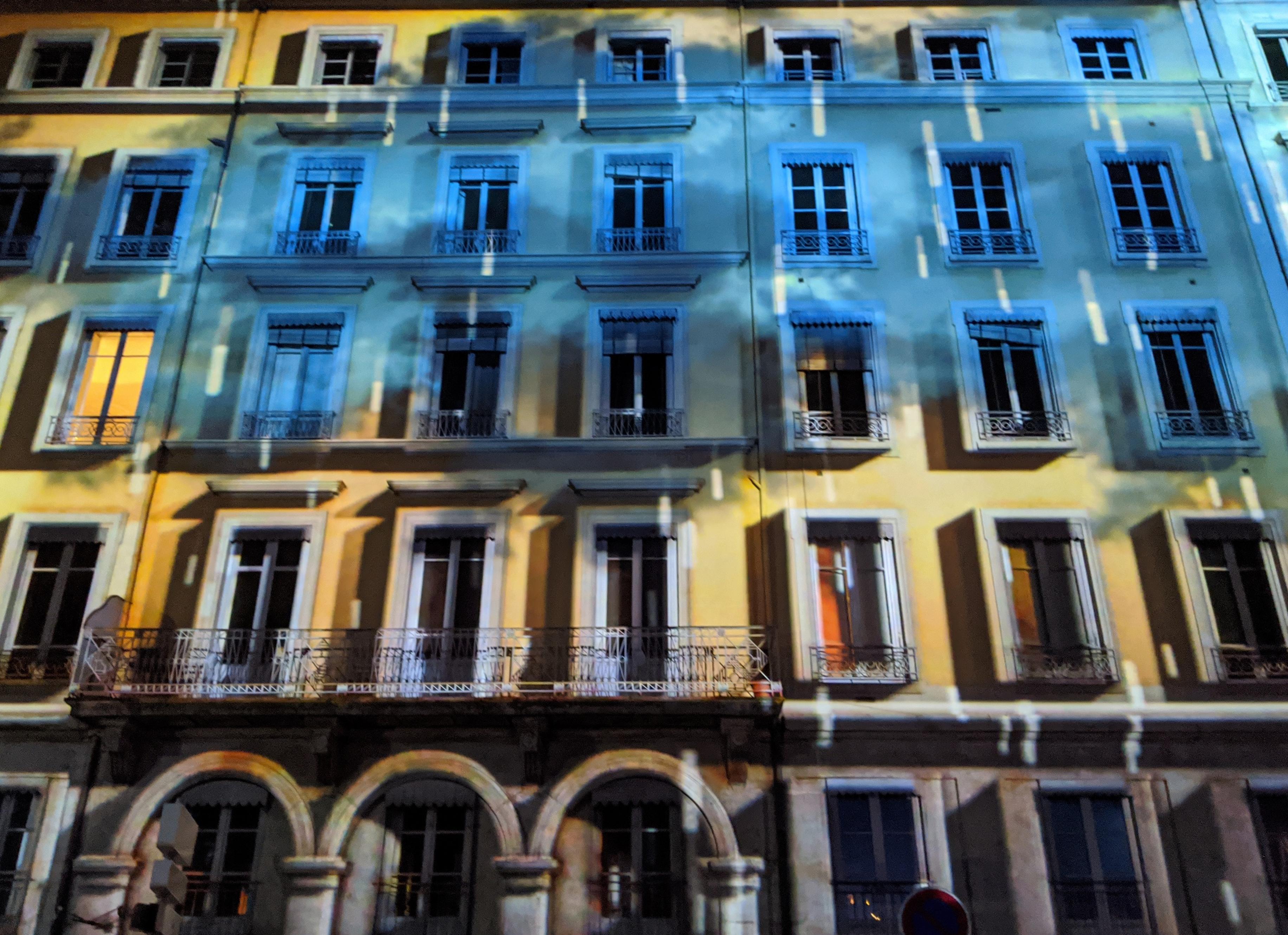
That said, a difficulty may arise in that rotated images may contain remnant black borders from the rotation. As such, when rotating to test for orientation, the candidate image must also be cropped to only contain image information. This signifies that every candidate image will have a different number of pixels, which will skew the metric. The solution is to weight the metric by the size of each image. The following images show the algorithm in action for a facade.
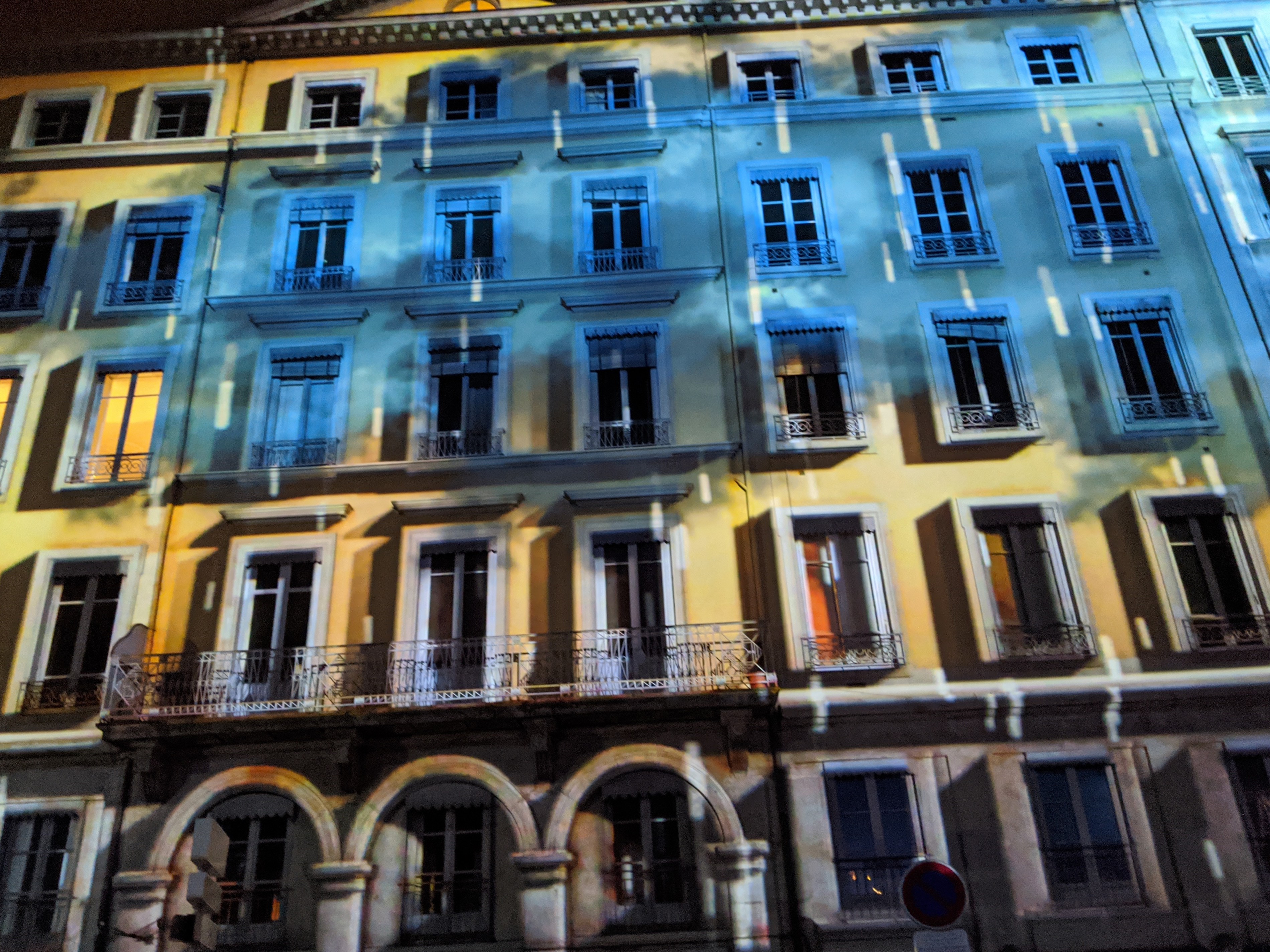
— original |
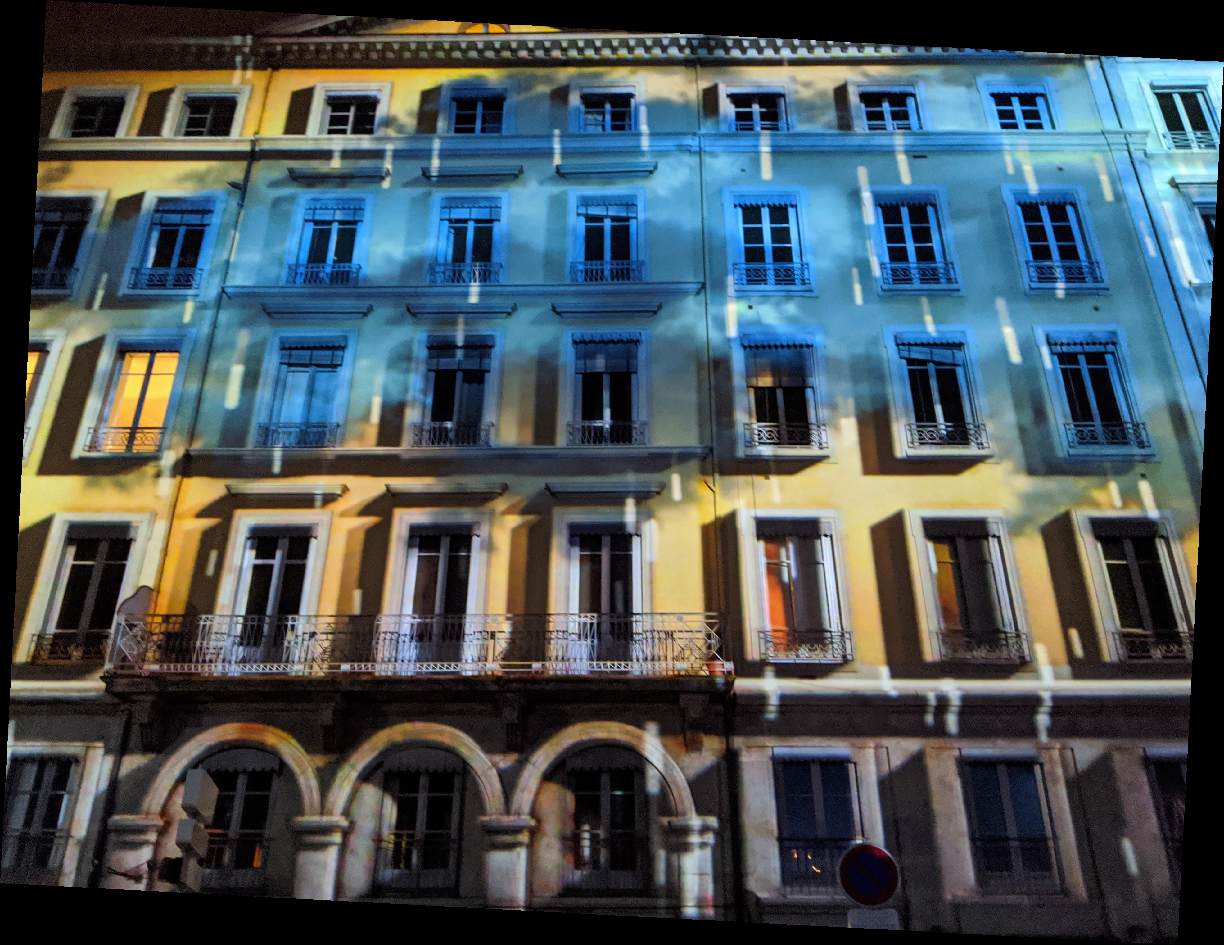
— -4° |
— -4°, cropped |
— original |

— -4° |
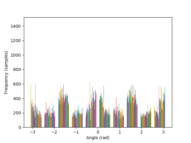
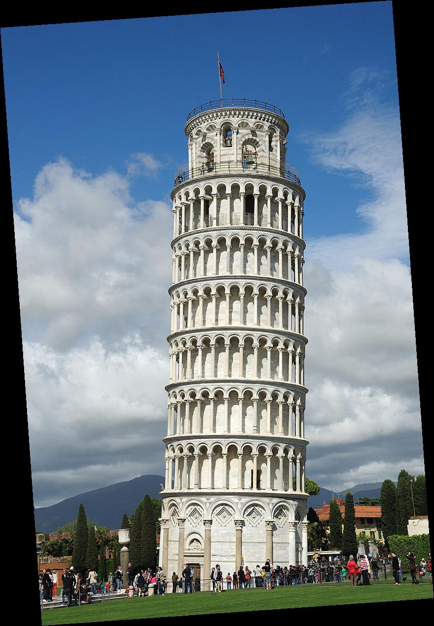
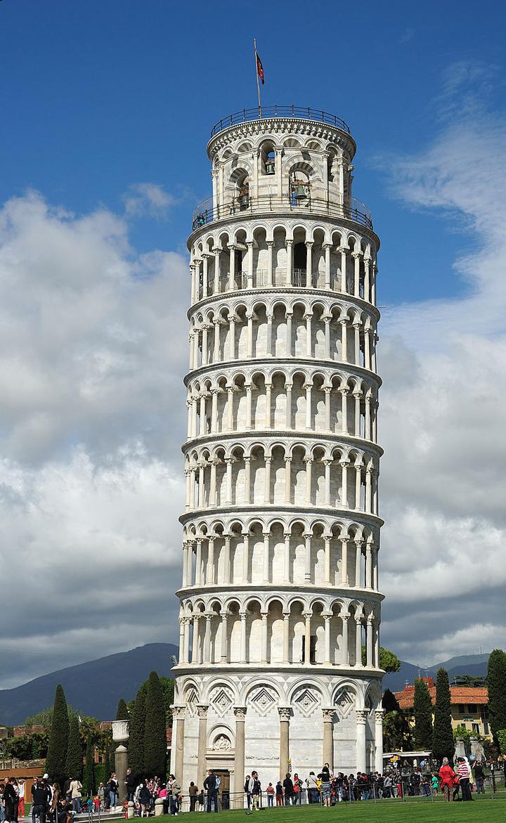
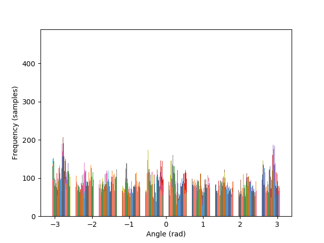
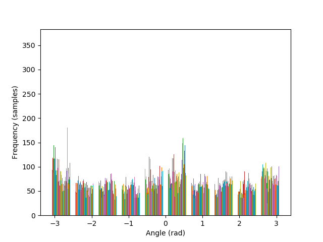
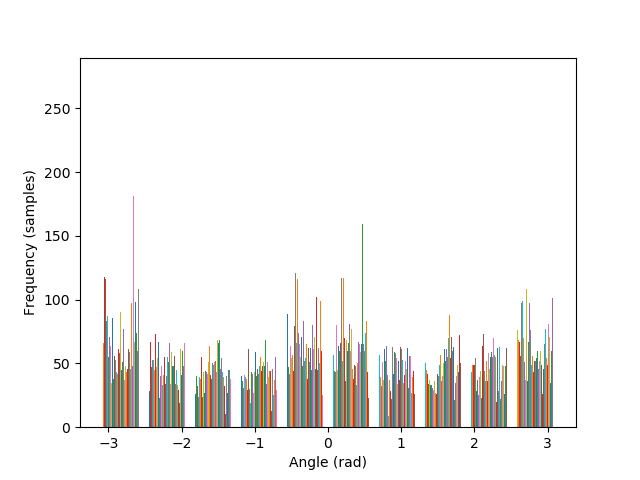
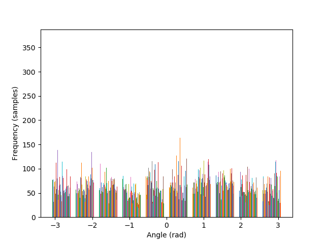
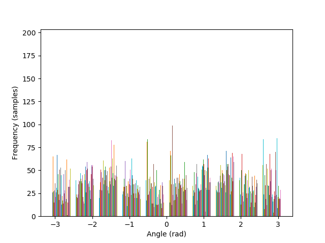
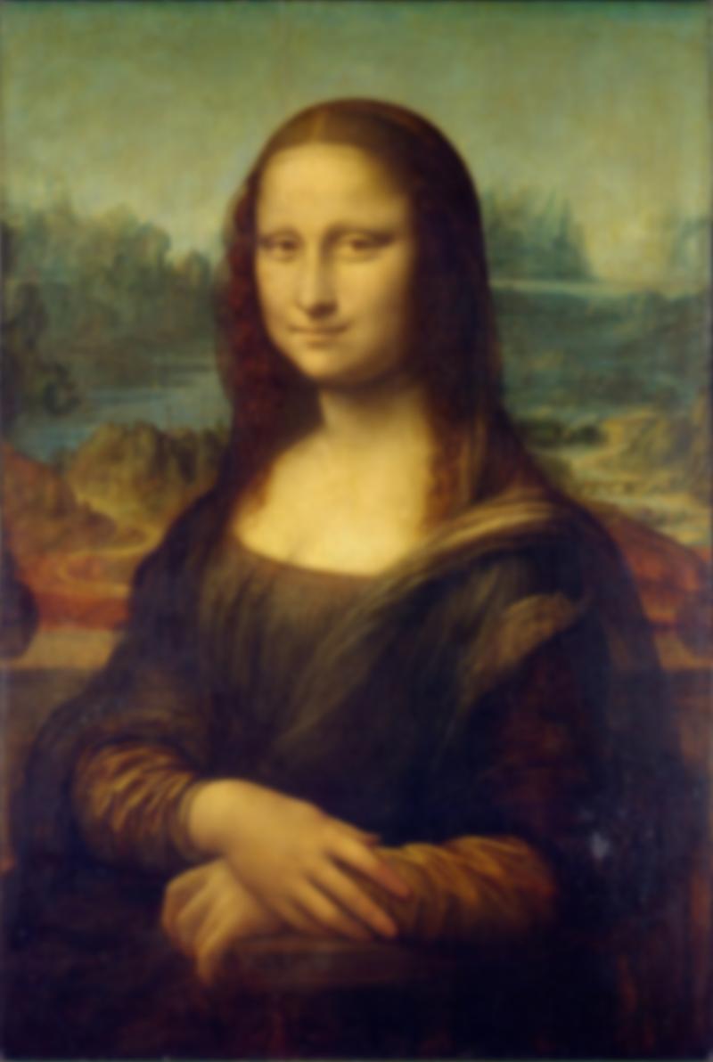
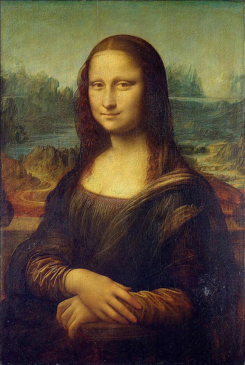
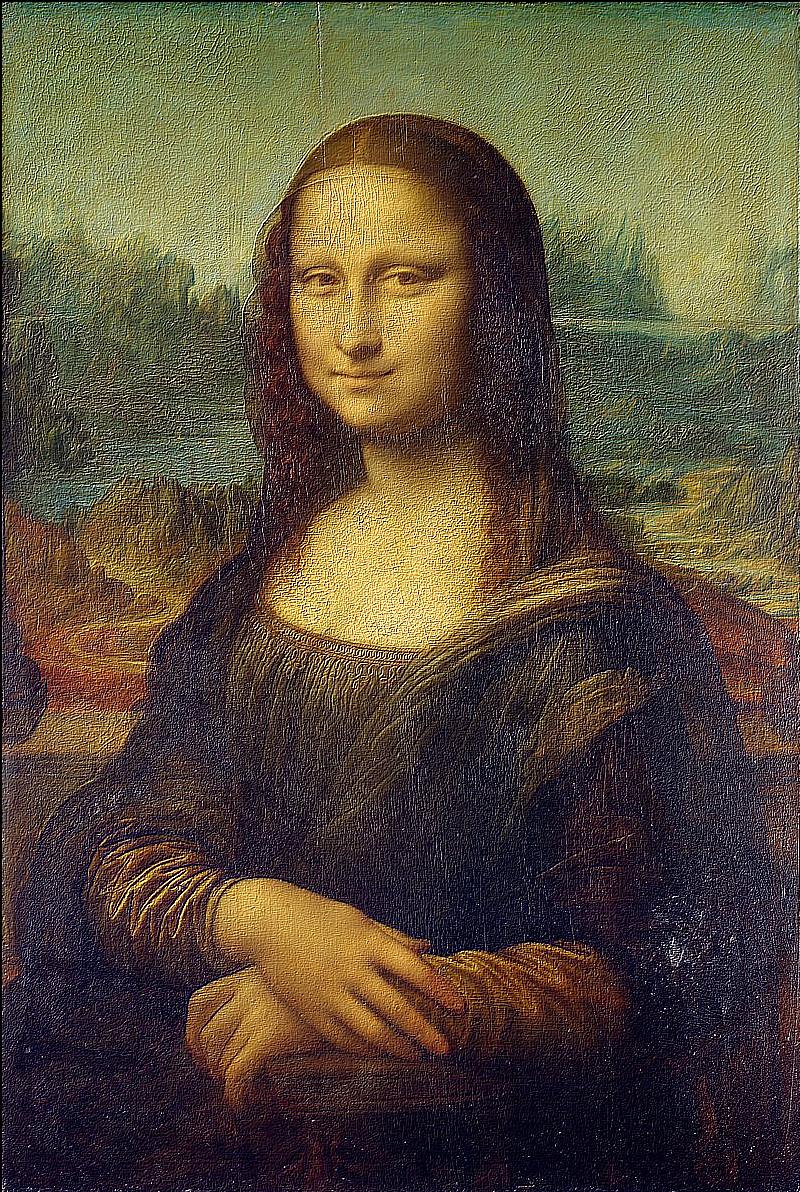
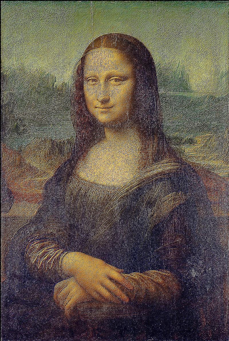
The algorithm is also able to straighten the legendary Tower of Pisa, and a badly rotated picture of Mona Lisa, with minimal error. As it can be seen in the histograms, the rotated images contain a greater number of pixels where the gradient is either 0, π, or, -π radians, compared to their original versions.
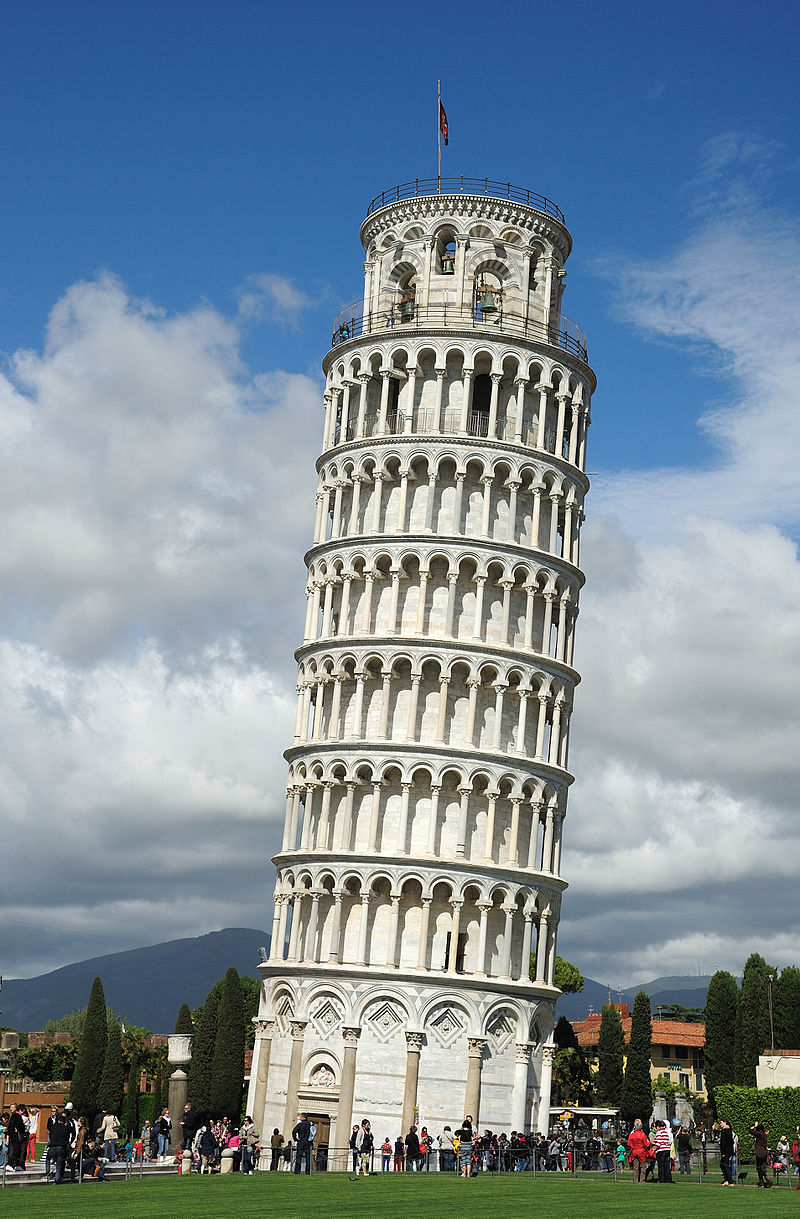
— original |
— 4° |
— 4°, cropped |
— original |
— 4° |
— original |
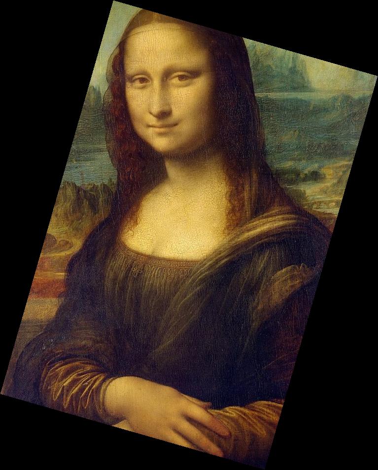
— -16° |
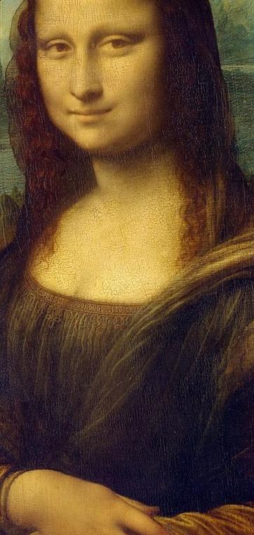
— -16°, cropped |
— original |
— -16° |
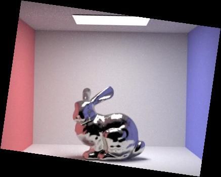
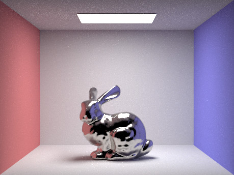
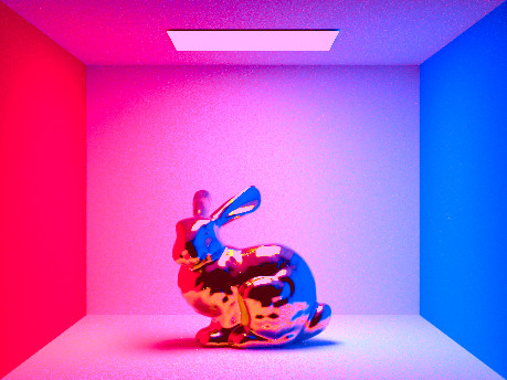
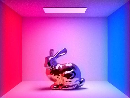
The algorithm is nevertheless far from perfect. Images that naturally contain curves, such as the following picture of a bunny rendered with platinum skin, result in failures.
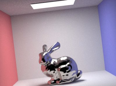
— self-render for CS184 |
— -8° |
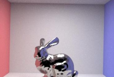
— -8°, cropped |
— (somewhat) original |
— -8° |
Speaking of failures, the algorithm cannot distinguish between rotations where the image is oriented according to how a human expects it, and one where it has been rotated by 90 or -90 degrees. Potential improvements to the algorithm (which however were outside of the scope of this project) include weighting the metric, or at least veryfying the edge cases, using feature detection.
— original |
— 10° (failure) |
— 10°, cropped |
— original |
— 10° |
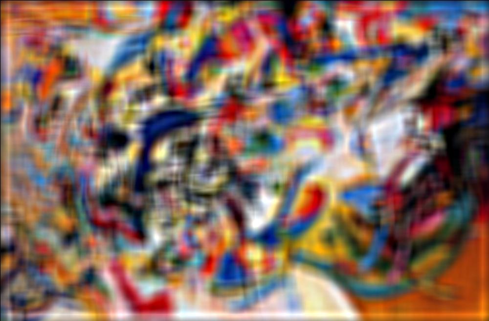
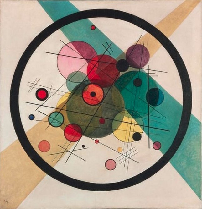
Finally, it is worth mentioning that certain cases exist where the algorithm, and even a potential one enhanced with feature detection, stands absolutely no chance of success. That said, it is doubtful whether a human stands much chance either. Certain things simply cannot be measured. Kadinsky's awe-provoking masterpiece, Composition VII is a compeling proof.
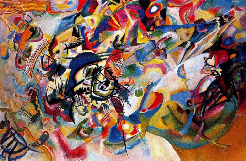
— Wassily Kadinsky (1913) |
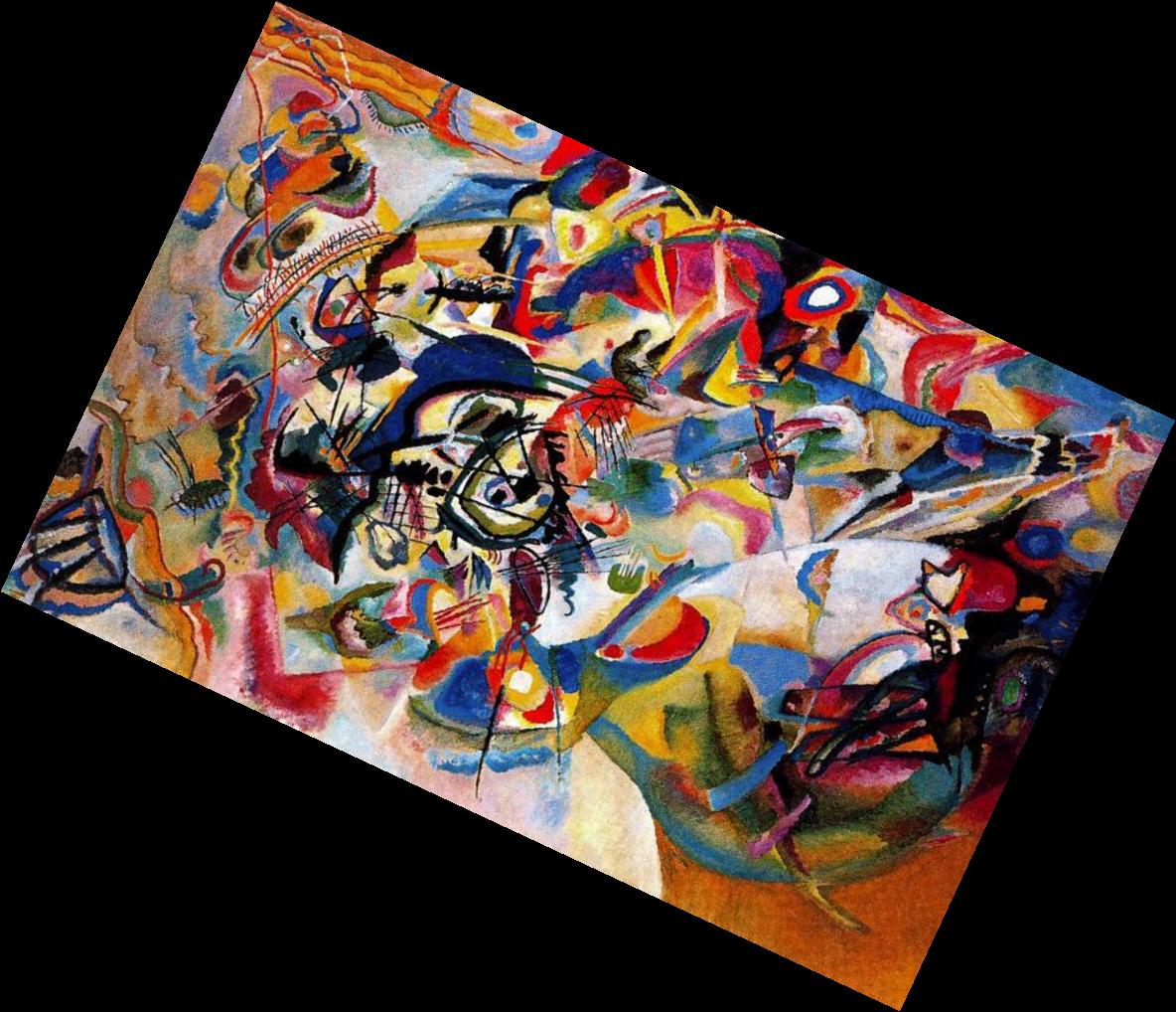
— -25° (failure?) |
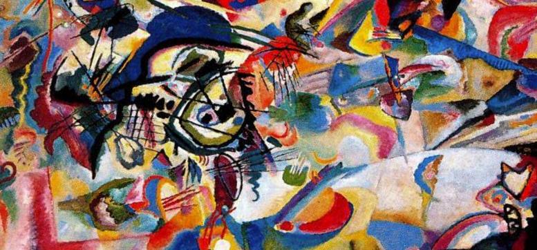
— -25°, cropped |
— original |
— -25° |
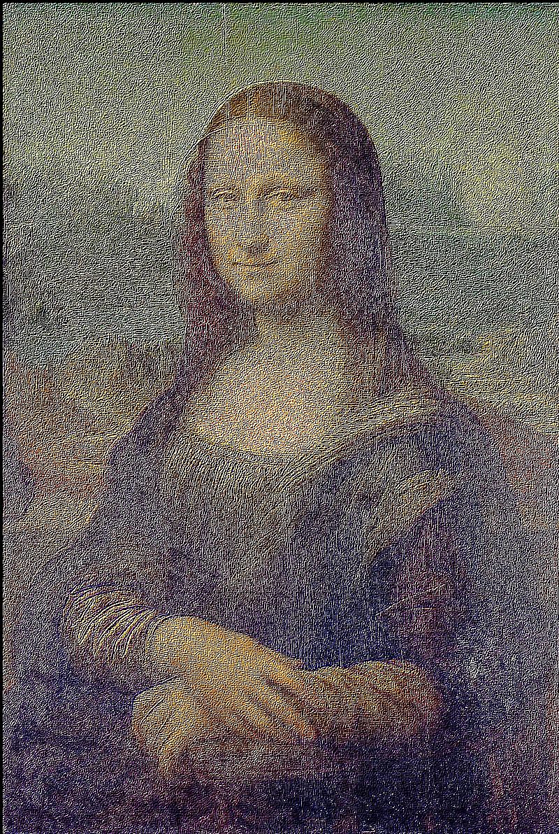
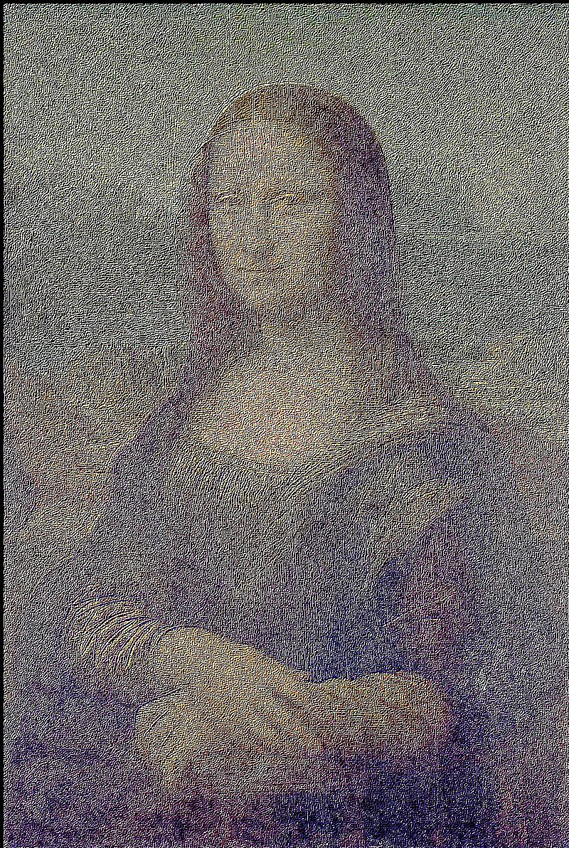
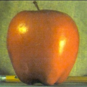
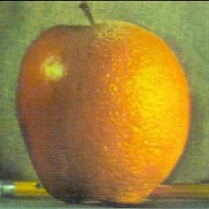
The Gaussian filter developed previously can find further use in image sharpening. A blurry image, in essence, is one that retained its low frequencies, yet had its high frequencies removed. When subtracted from the original image, the blurry (low frequencies) image yields a very crisp (high frequencies) image. The original image can be sharpened by simply adding it up to the crisp image, factored to taste.
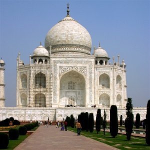
— original |
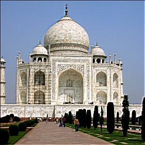
— unsharp mask |

— gaussian blur |
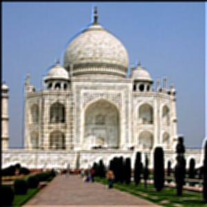
— unsharp mask on gaussian blur |
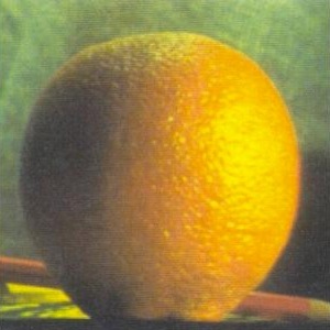
Notice the unsharp mask can make a relatively low resolution image appear to be higher resolution, and even enhance perceived color. However, it is by no means magical. Images that are naturally blurry (or became blurry) will remain so.

— original |

— unsharp mask (notice colors) |

— gaussian blur |
— unsharp mask on gaussian blur |
— original |
— unsharp mask (notice details) |
— gaussian blur |
— unsharp mask on gaussian blur |
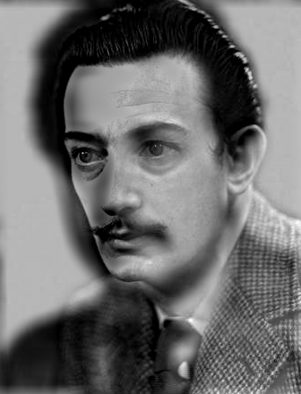
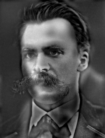
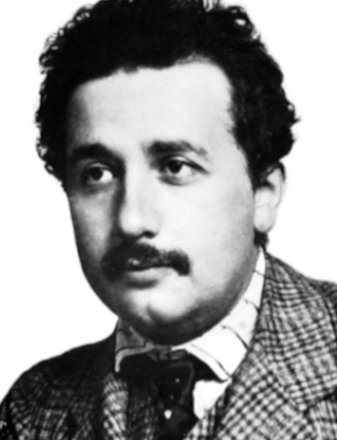
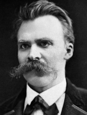
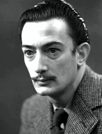
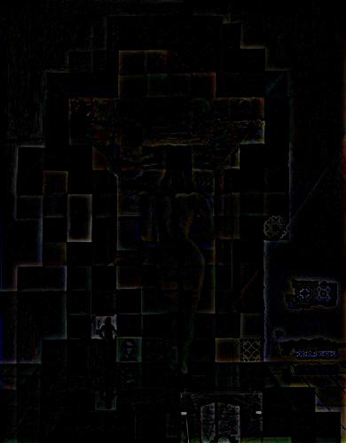
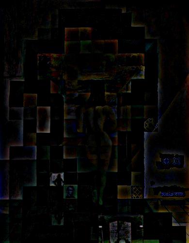
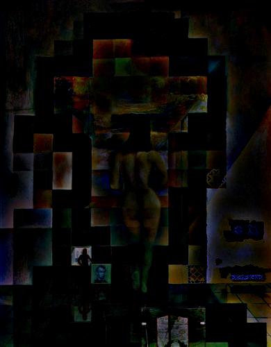
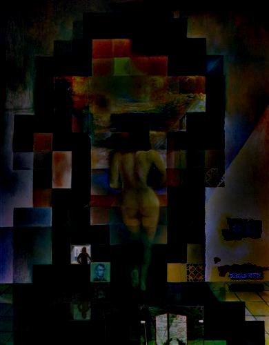
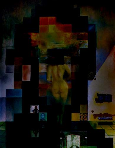
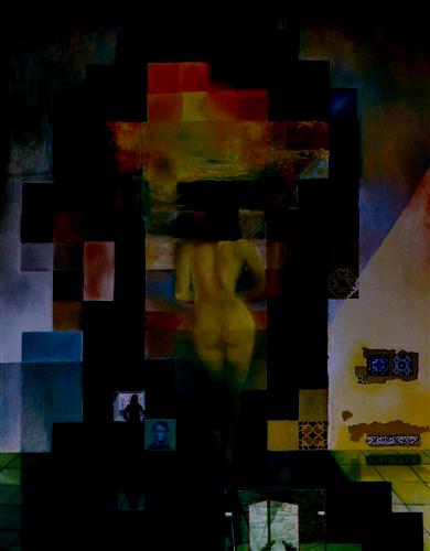
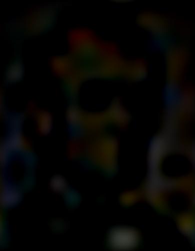
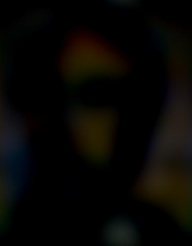
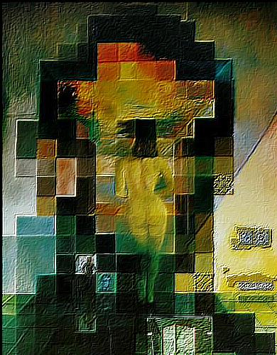
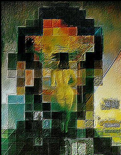
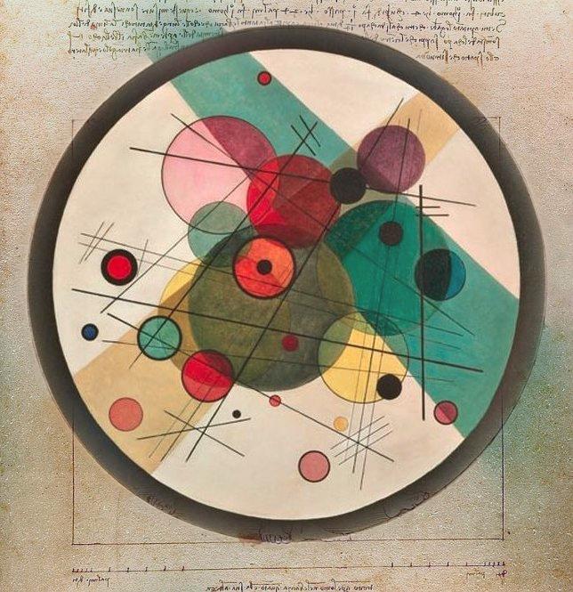
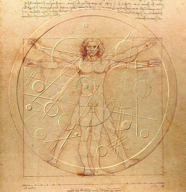
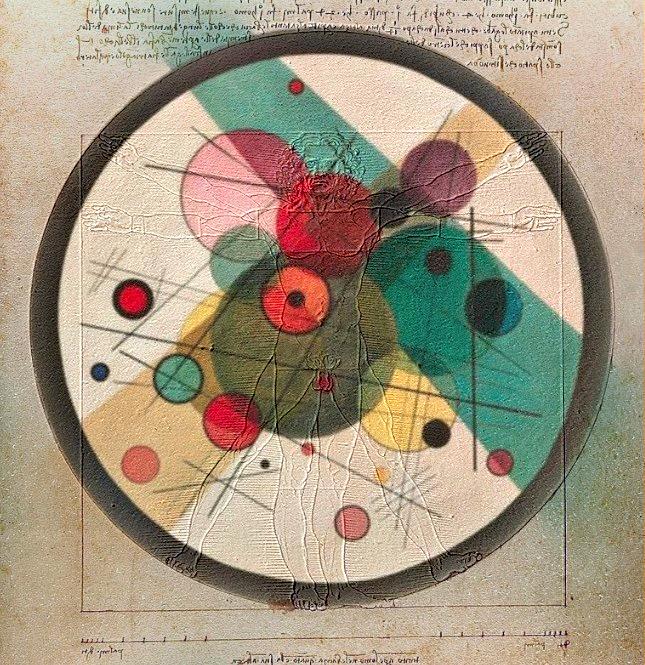
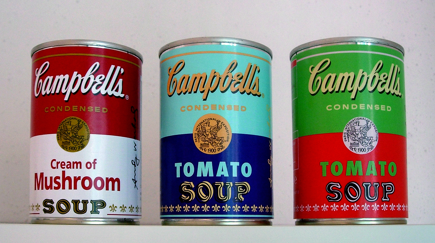
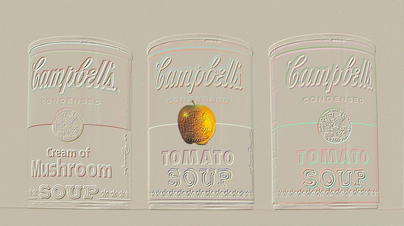
Two advanced applications of the Gaussian Blur are Hybrid Images (Oliva, Torralba, Schyns, SIGGRAPH 2006) and Multiresolution Blending (Burt and Adelson, ACM Transactions on Graphics 1983). Hybrid Images are images containing two scenes within one, and which appear selectively based on the viewer's distance. Multiresolution Blending referes to a technique of taking a patch from one image, and seamlesly aking it appear as an organic part of another.
The algorithms of this part were implemented exactly as outlined by their authors. As a sole exception, in multiresolution blending similar resolution stacks were used over pyramids to preserve as much information as possible. Furthermore, to speed up the filtering process, every image was first converted to its frequency domain with a Fast Fourier Transform, and then, once the desired filter had been applied, inverted back to its spatial domain. The following images demonstrate the results.
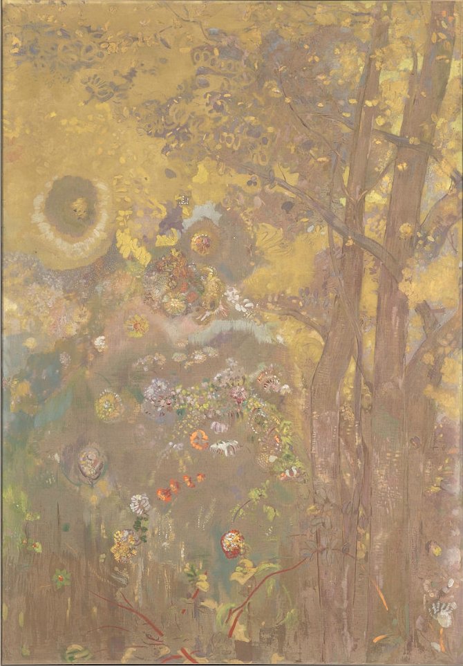
— Odilon Redon (1901) |
|

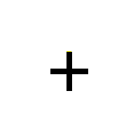
— Yves Klein (1962) |

|
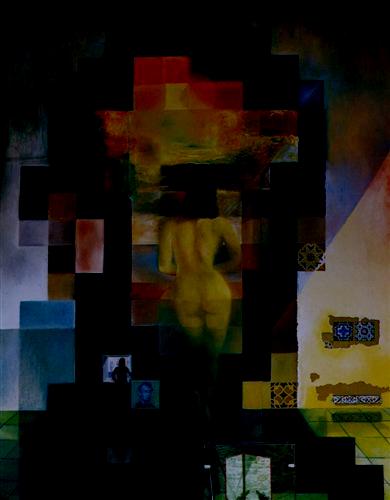
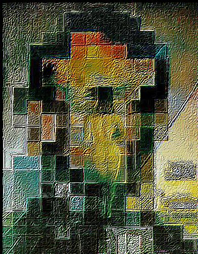
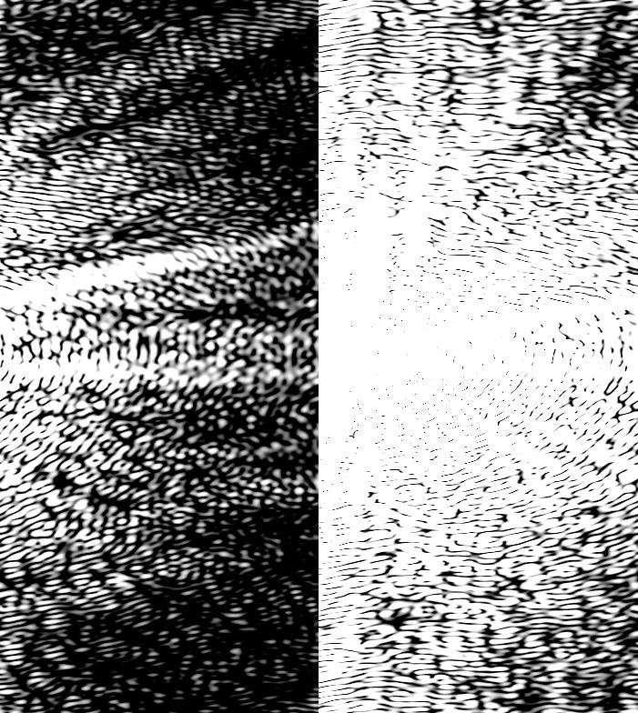
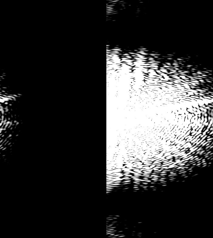
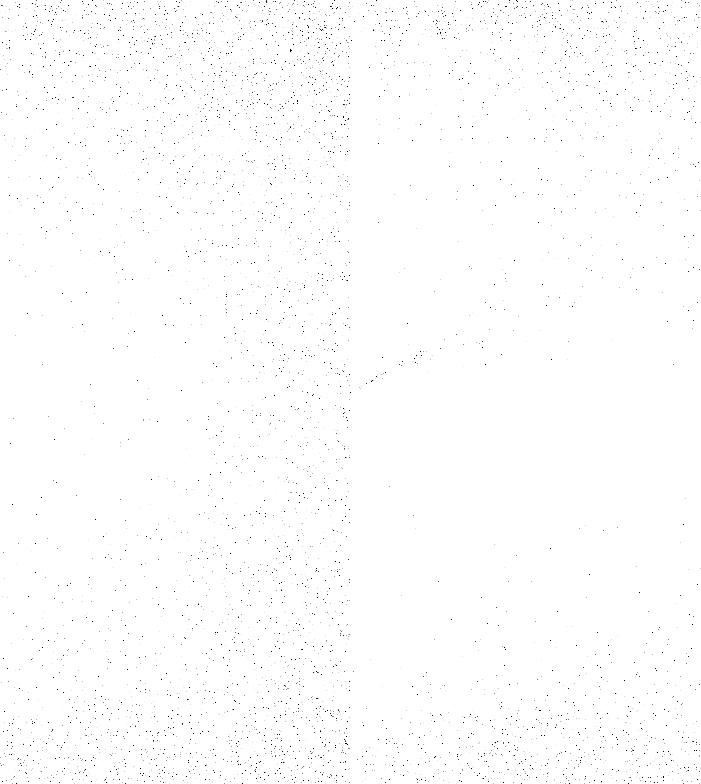
— Nature Plastique |
— low frequencies |
|
— high frequencies |
|
|
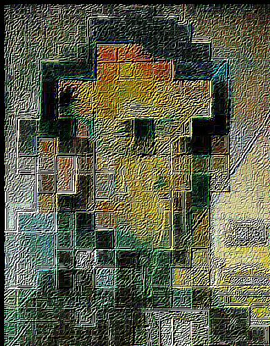
— failure (but an absolutely beautiful one!) |
— low frequencies |
|
— high frequencies |
|
|
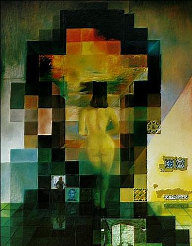
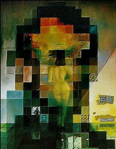
— when the features of the images blended are extremely similar, the effect is inevident |
|

|
|
|
|
|
|
— low frequencies |
|
— high frequencies |
|
|
|
— hybrid |

— frequency domain |

— frequency domain |

— gaussian |

— laplacian |

— frequency domain |
|
— low frequencies |
|
— high frequencies |
|
|
|
— hybrid |

— gaussian, level 1 |

— gaussian, level 2 |

— gaussian, level 3 |

— gaussian, level 4 |

— gaussian, level 5 |
|
— low frequencies |
|
— high frequencies |
|
|
|
— hybrid |
— laplacian, level 1 |
— laplacian, level 2 |
— laplacian, level 3 |
— laplacian, level 4 |
— laplacian, level 5 |

— gaussian, level 0 |

— gaussian, level 1 |

— gaussian, level 2 |
— gaussian, level 3 |

— gaussian, level 4 |
— gaussian, level 5 |
— gaussian, level 6 |

— gaussian, level 7 |

— gaussian, level 8 |

— gaussian, level 9 |

— laplacian, level 0 |
— laplacian, level 1 |
— laplacian, level 2 |
— laplacian, level 3 |
— laplacian, level 4 |
— laplacian, level 5 |
— laplacian, level 6 |
— laplacian, level 7 |
— laplacian, level 8 |
— laplacian, level 9 |
— bandpass, level 0 |

— bandpass, level 1 |
— bandpass, level 2 |
— bandpass, level 3 |
— bandpass, level 4 |
— bandpass, level 5 |
— bandpass, level 6 |
— bandpass, level 7 |

— bandpass, level 8 |

— bandpass, level 9 |
— sharpen, level 0 |
— sharpen, level 1 |
— sharpen, level 2 |
— sharpen, level 3 |
— sharpen, level 4 |
— sharpen, level 5 |
— sharpen, level 6 |
— sharpen, level 7 |
— sharpen, level 8 |
— sharpen, level 9 |

— gaussian, level 0 |

— gaussian, level 1 |

— gaussian, level 2 |
— gaussian, level 3 |

— gaussian, level 4 |

— gaussian, level 5 |
— gaussian, level 6 |

— gaussian, level 7 |

— gaussian, level 8 |

— gaussian, level 9 |
— laplacian, level 0 |
— laplacian, level 1 |
— laplacian, level 2 |
— laplacian, level 3 |
— laplacian, level 4 |
— laplacian, level 5 |
— laplacian, level 6 |
— laplacian, level 7 |
— laplacian, level 8 |
— laplacian, level 9 |

— bandpass, level 0 |
— bandpass, level 1 |
— bandpass, level 2 |
— bandpass, level 3 |
— bandpass, level 4 |
— bandpass, level 5 |
— bandpass, level 6 |

— bandpass, level 7 |
— bandpass, level 8 |

— bandpass, level 9 |
— sharpen, level 0 |
— sharpen, level 1 |
— sharpen, level 2 |
— sharpen, level 3 |
— sharpen, level 4 |
— sharpen, level 5 |
— sharpen, level 6 |
— sharpen, level 7 |
— sharpen, level 8 |
— sharpen, level 9 |
— Wassily Kadinsky (1923) |
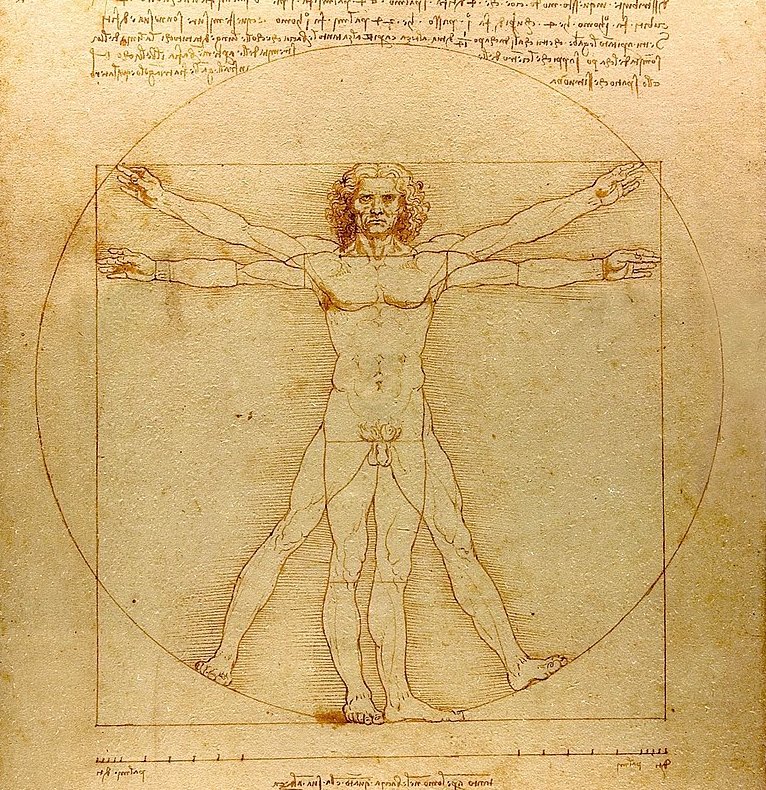
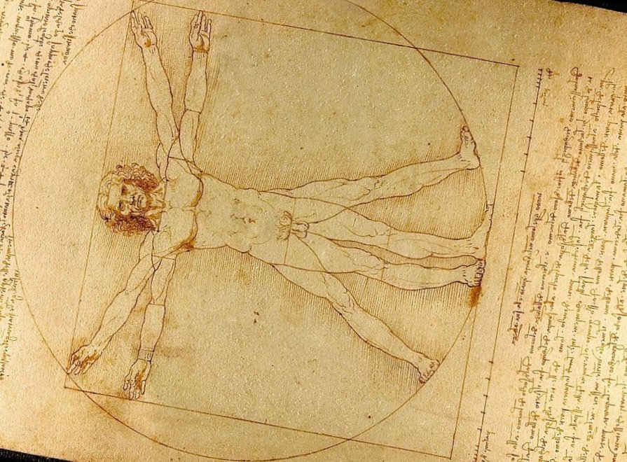
— Leonardo Da Vinci (c. 1490) |
— Mechanics |
— laplacian, level 0 |

— laplacian, level 1 |

— laplacian, level 2 |

— laplacian, level 3 |

— laplacian, level 4 |

— laplacian, level 5 |

— laplacian, level 6 |

— laplacian, level 7 |

— laplacian, level 8 |

— laplacian, level 9 |

— mask, level 0 |

— mask, level 1 |

— mask, level 2 |

— mask, level 3 |

— mask, level 4 |

— mask, level 5 |

— mask, level 6 |

— mask, level 7 |

— mask, level 8 |

— mask, level 9 |

— applied mask, level 0 |

— applied mask, level 1 |

— applied mask, level 2 |

— applied mask, level 3 |

— applied mask, level 4 |

— applied mask, level 5 |

— applied mask, level 6 |

— applied mask, level 7 |

— applied mask, level 8 |

— applied mask, level 9 |
|
— low frequencies |
— high frequencies |
— |
|
— low frequencies |
— high frequencies |
— Διόνυσος |
— top |
— bottom |
— |
— laplacian, level 0 |

— laplacian, level 1 |
— laplacian, level 2 |
— laplacian, level 3 |
— laplacian, level 4 |
— laplacian, level 5 |
— laplacian, level 6 |
— laplacian, level 7 |
— laplacian, level 8 |

— laplacian, level 9 |
— mask, level 0 |
— mask, level 1 |
— mask, level 2 |
— mask, level 3 |
— mask, level 4 |
— mask, level 5 |
— mask, level 6 |

— mask, level 7 |

— mask, level 8 |

— mask, level 9 |
— applied mask, level 0 |

— applied mask, level 1 |
— applied mask, level 2 |
— applied mask, level 3 |
— applied mask, level 4 |
— applied mask, level 5 |
— applied mask, level 6 |

— applied mask, level 7 |

— applied mask, level 8 |

— applied mask, level 9 |
— John Leffmann (2015) |
— |
— frequency domain |

— frequency domain |
— gaussian |
— laplacian |

— frequency domain |

— level 0 |

— level 5 |

— level 9 |