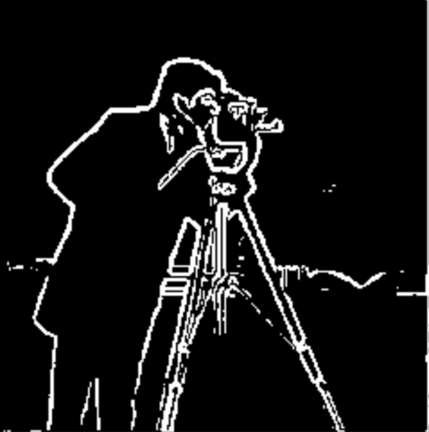
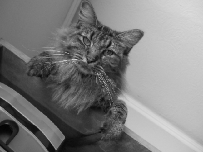
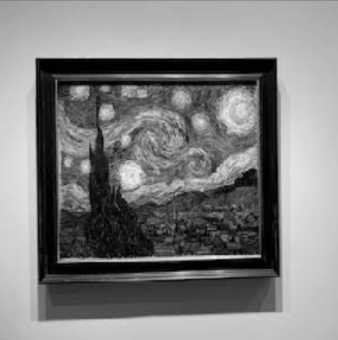
In this section, we used our finite difference operator on the cameraman image to generate two derivative images with respect to the x-axis and y-axis. We then combined the two images using the gradient magnitude equation, which is the square root of the added squares of the derivatives, to generate the edge image. Lastly, I binarized the result of this to remove noise. Unfortunately, due to the amount of noise in the resulting edge image, the binarization threshold numbers had to be quite aggresive in order to remove most of it, causing a loss of some detail.
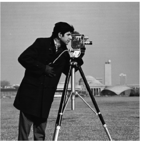
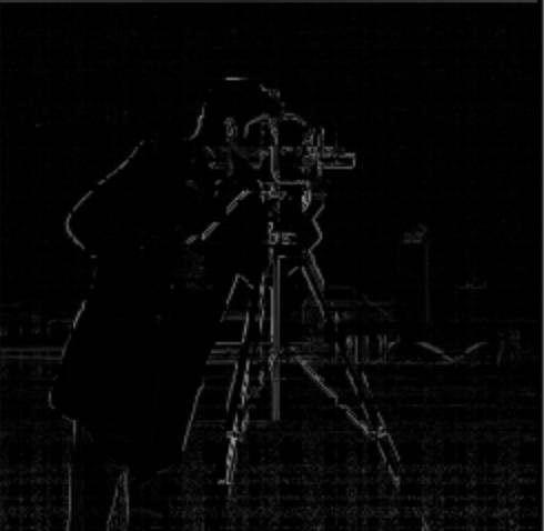
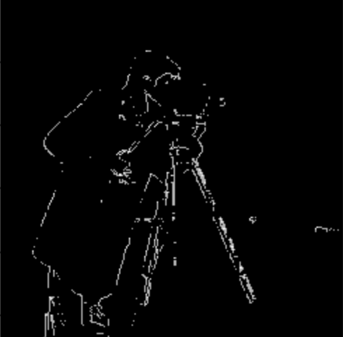
We convolved the cameraman image to find the edges. To get an edge image, we first got the partial derivative in x of the image by convolving it with the filter [[1,-1]]. Similarly we got the partial derivative in y of the image by convolving it with [[1],[-1]]. We then used the gradient magnitude equation to combine the two images (the square root of the added squares of the derivatives), which finds the edges of the images. However, this image of the edges produced very noisy results, with a lot of unclear edges. Therefore, we binarized the edges to remove noise.
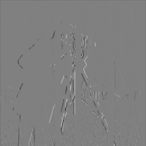
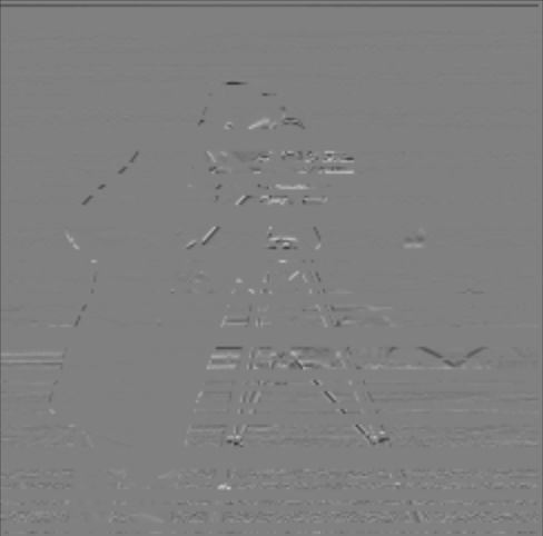
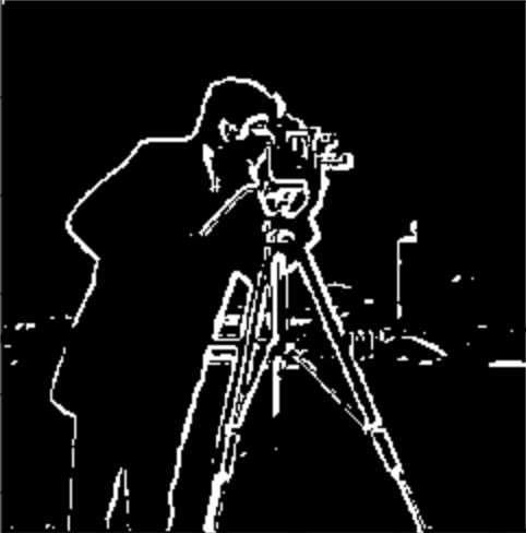
In the last part, there was a lot of noise even after binarizing the edges. Therefore, we applied a gaussian filter (8x8, sigma = 2) in order to “smooth” out the image, which makes it easier to detect edges. There are two methods of doing this, but both produce the same result.
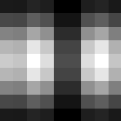
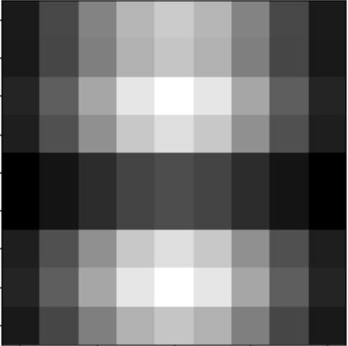
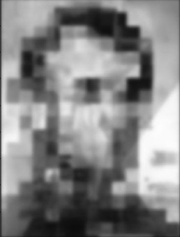
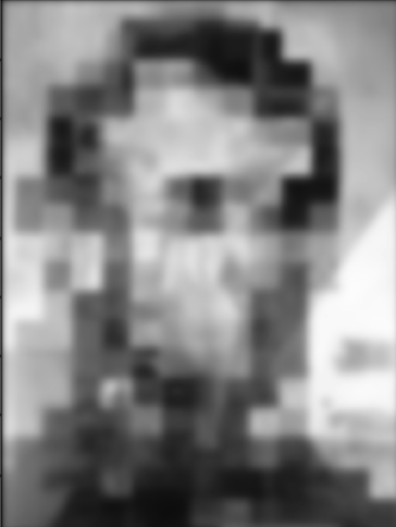
Method 1 involves finding the convolution of the gaussian filter with [[-1, 1]] and [[-1],[1]] and then using that result to convolve with the actual cameraman image. Method 1 is better in bigger computations, because it is faster. You can reuse the constant convolved gaussian with [[-1, 1]] and [[-1],[1]]. Method 2 involves finding the convolution of the gaussian filter with the image and then using that result to convolve with the [[-1, 1]] and [[-1],[1]] . As you can see in the resulting images below, both methods produce the same result.
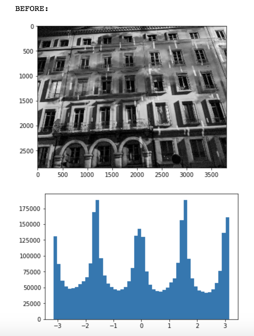
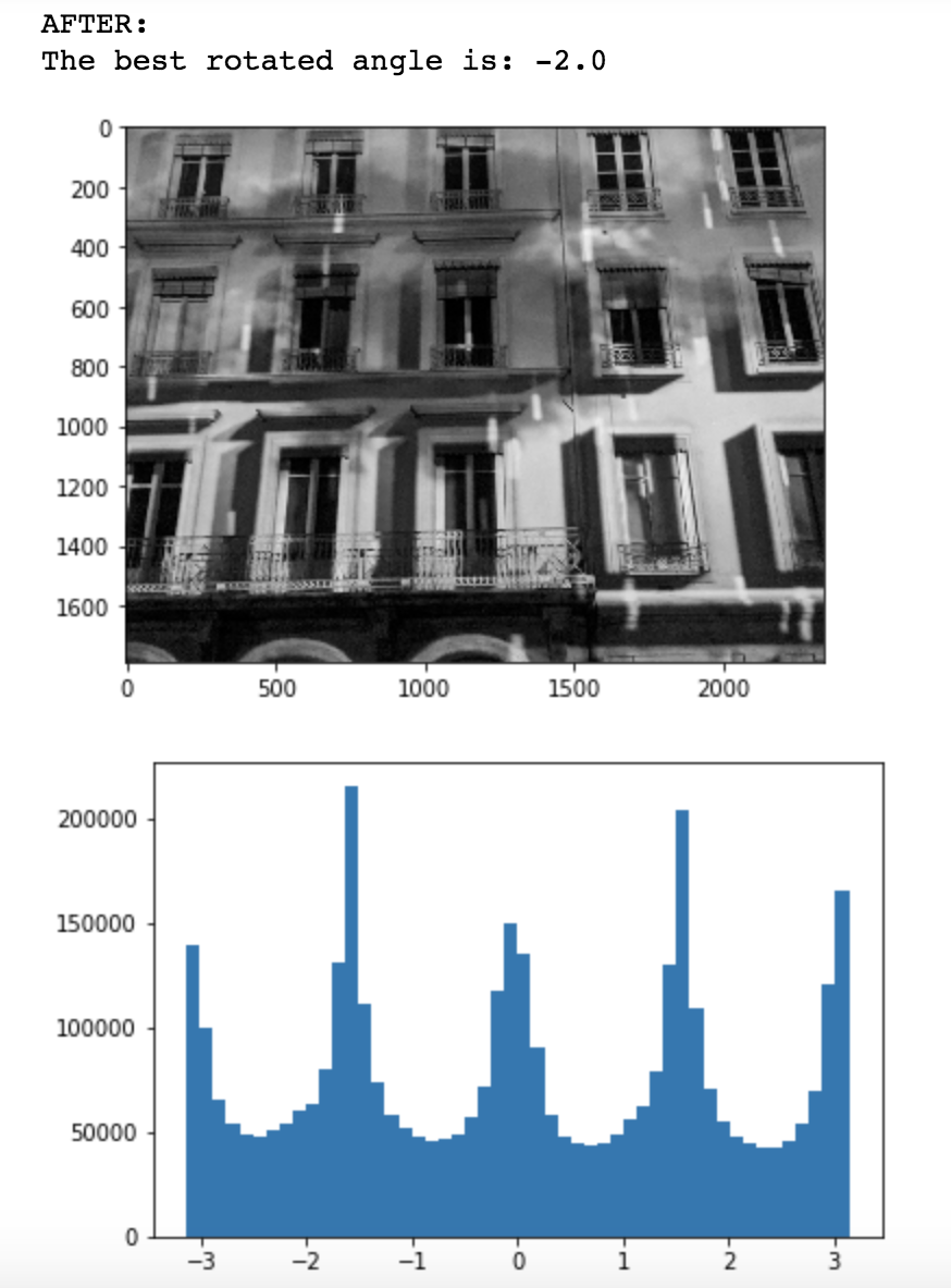
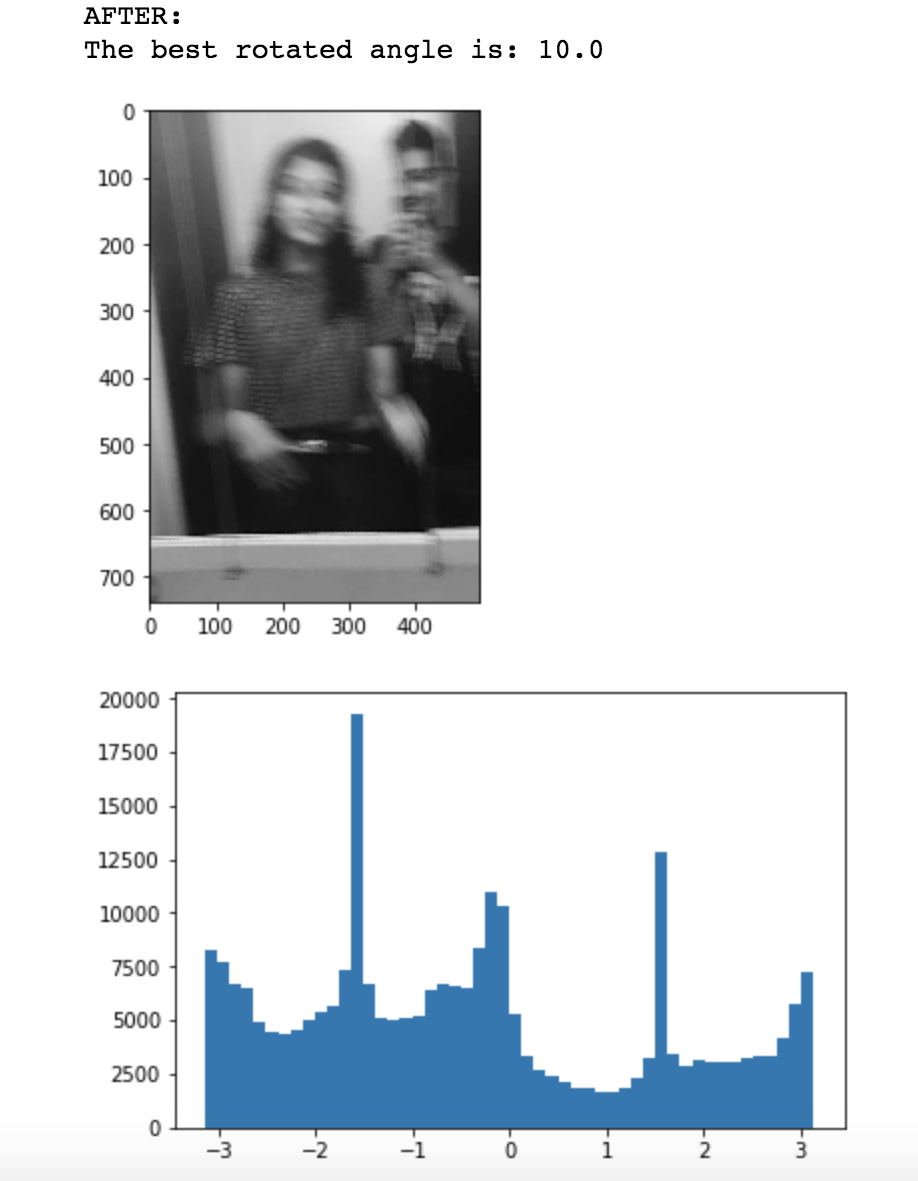
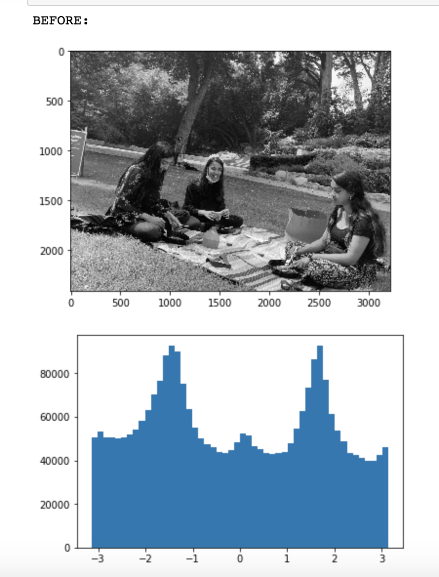
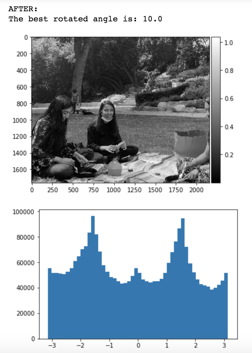
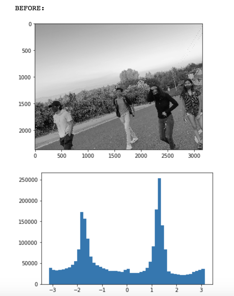
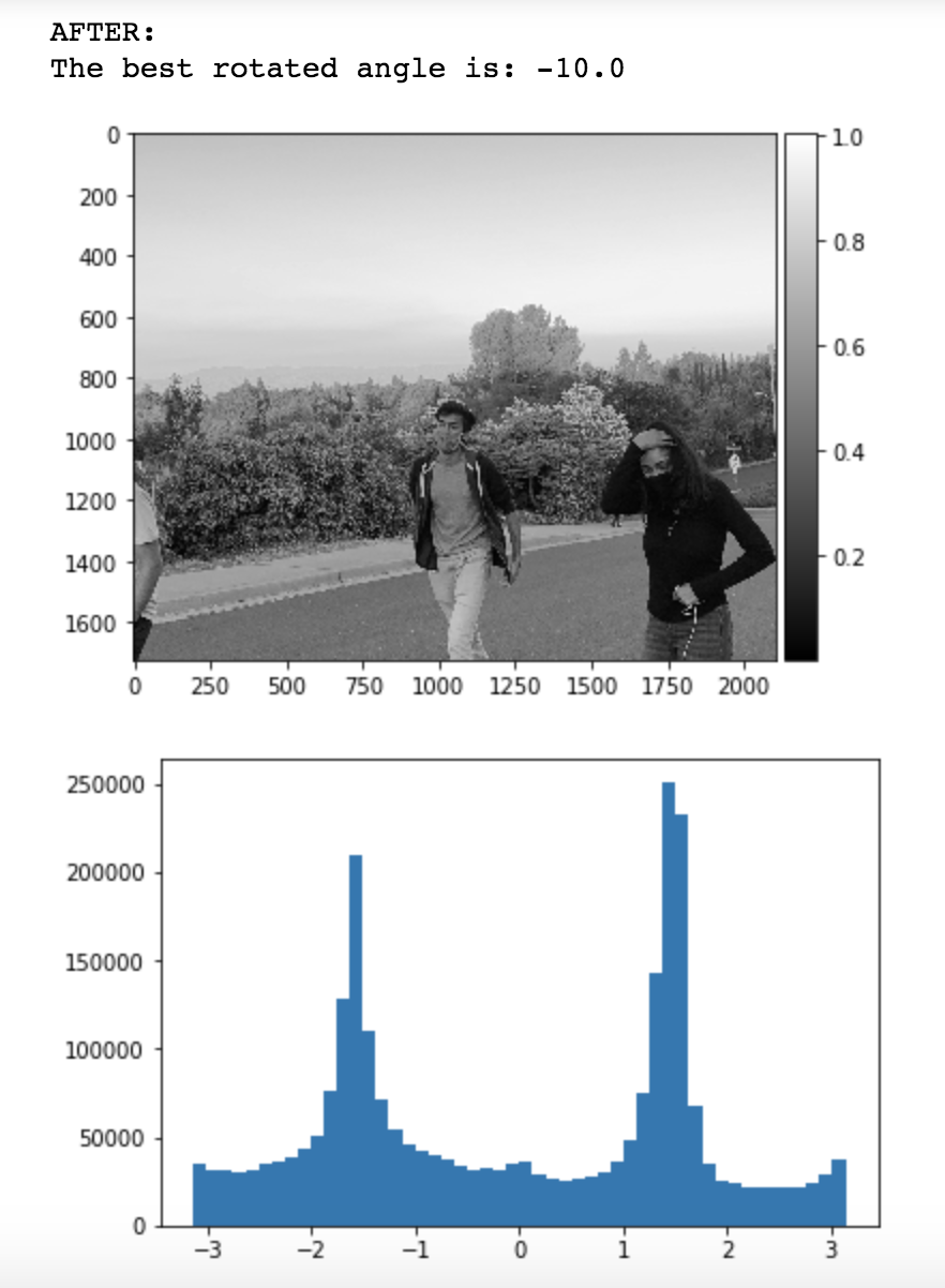
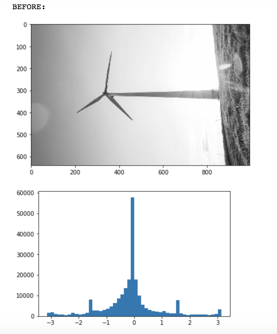
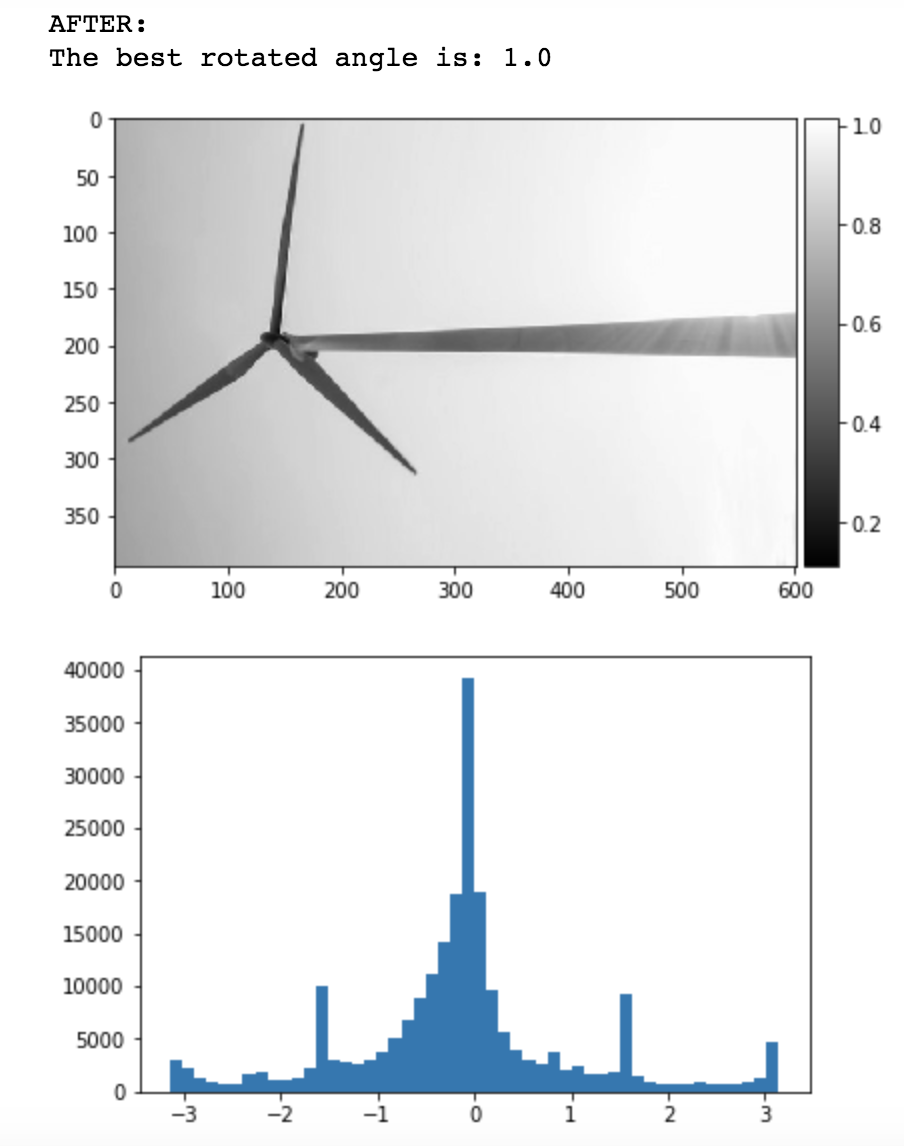
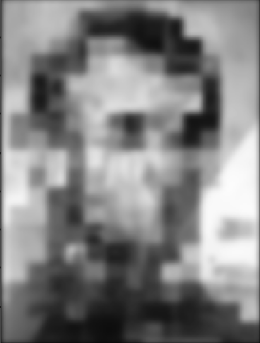
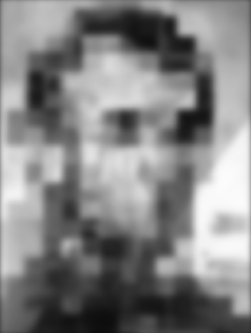
Now, we want to take images that are slightly rotated and rotate them to a certain degree such that the image appears straight. We used our gradient and edge detection methods from parts 1.1 and 1.2 to help create a function that automatically straightens our images.
This is achieved by rotating the image by various angles and counting the number of vertical and horizontal edges in each rotated image. We convolve each rotated image with the gaussian filter to smooth it out, so it’s easier to detect edges. For each rotated image, we crop it (so that the black surroundings from the rotation do not appear) and we then count the number of horizontal and vertical edges. We keep track of the angle that resulted in the highest number of horizontal and vertical edges in the rotated image.
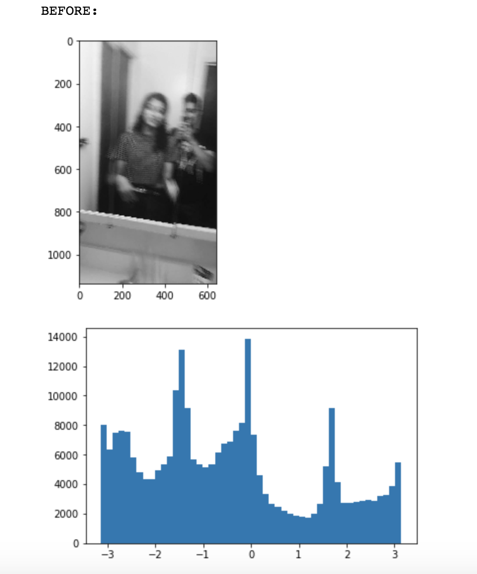
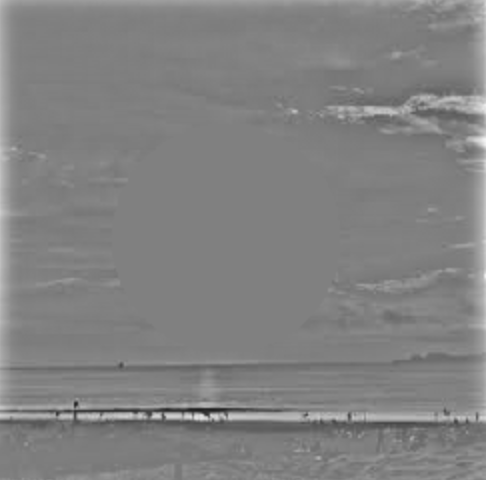
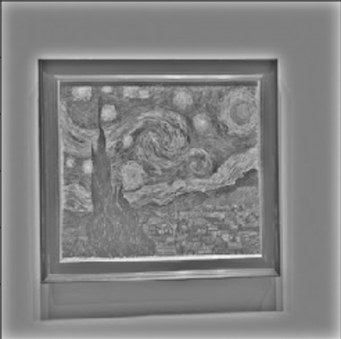
I tried 21 different angles from each image, ranging from -10 to 10 degrees. I then applied this rotation algorithm on four different images, and they all worked pretty well. There was one failure case, where the image did not straighten at all.
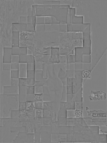
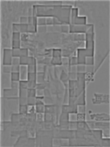
I display the histogram for each image rotated at it’s “best” angle. The histograms count the number of edges at various degrees for each image rotated at its “best” angle.
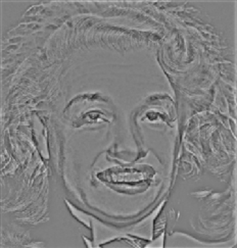
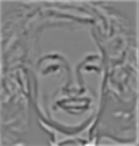
Now, we want to be able to sharpen images. We achieve this by blurring an image using a low-pass gaussian filter. Then, we subtract the blurred image from the original image to isolate the high frequencies in the image. This result contains an image with a lot of details, so we multiply the image with high frequencies by an alpha and add it back to the original image to create the sharpened image.
Here, I took a normal clarity image and blurred it using a gaussian filter. I then sharpened it using the method described above. It worked well.
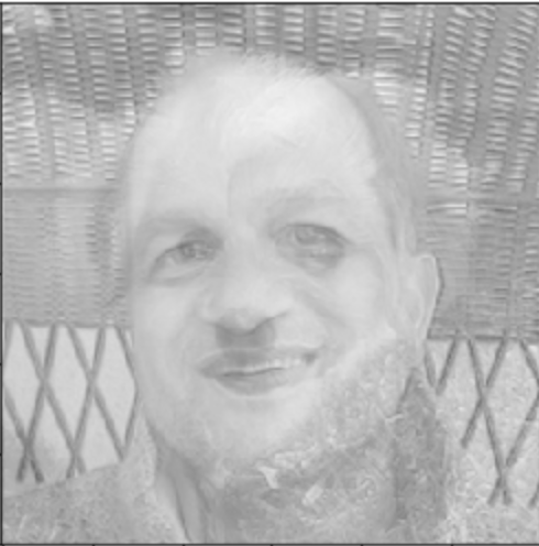
Here, I took a blurry image and tried to sharpen it. It didn't work that well and simply appeared a little darker. This is probably because the image was too shaky, rather than blurry to begin with.
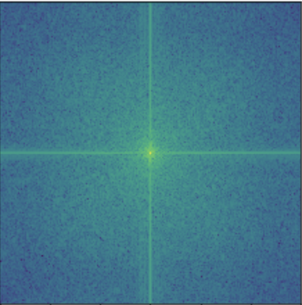
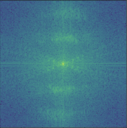
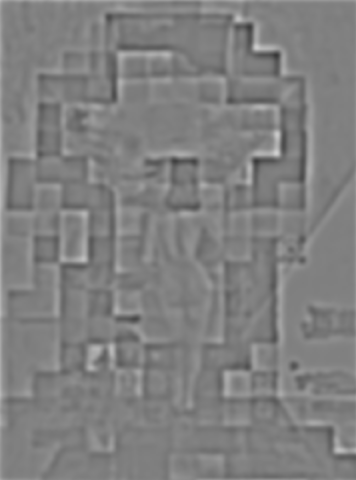
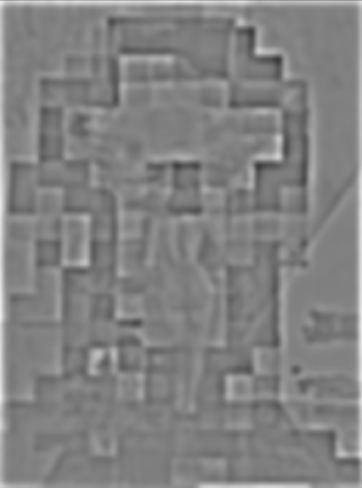
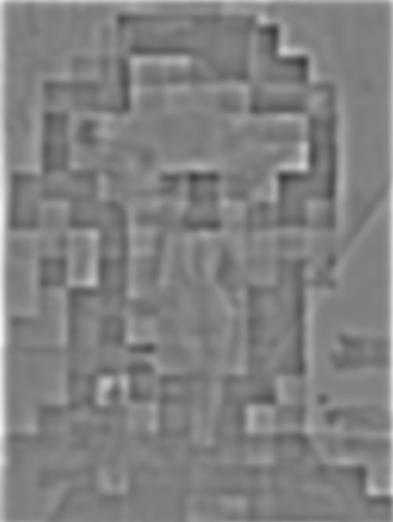
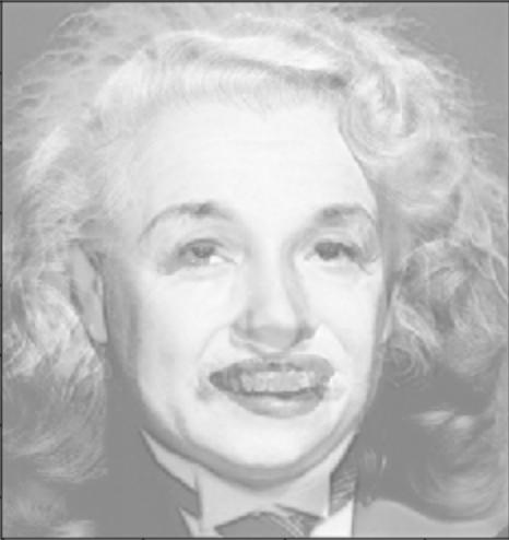
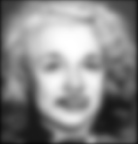
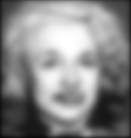
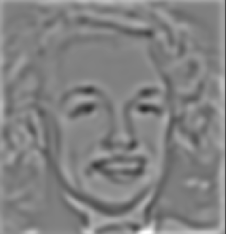
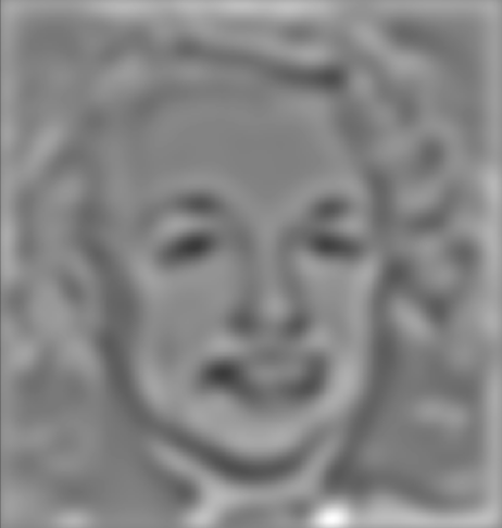
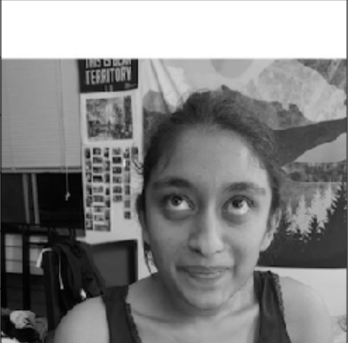
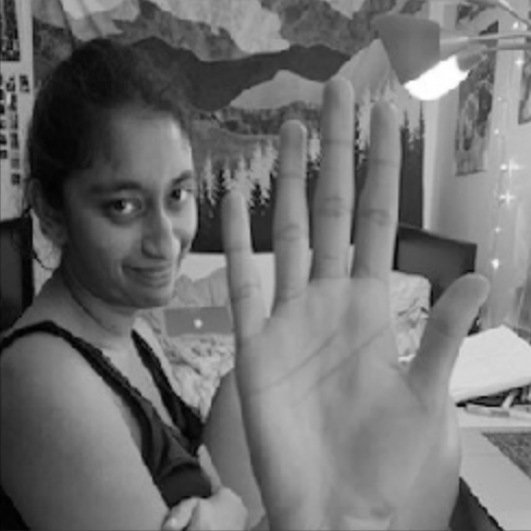
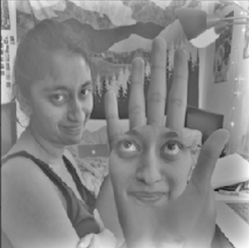
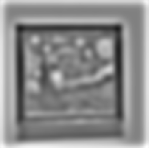
Now, we try to morph images together through this concept of “hybrid images.” This idea involves combining two images that appear different depending on where you are standing. If you’re standing close to the image, you will see the high_frequencies and if you’re standing far, you will see the lower frequencies. We create this hybrid image in a way that presents one image at lower frequencies, so you only see it from afar. And the other image at higher frequencies is only seen from afar.
The way we achieved this is by first aligning the images. My macbook didn’t have a high enough version to be able to use this alignment function, so I manually aligned it and used those manually aligned images. We apply two different gaussian filters to each image to blur them. With one image, we simply use the blurred version in our hybrid image. With the other, we use the blurred image to compute the sharpened image. We then sum up/average these images to create this hybrid image.
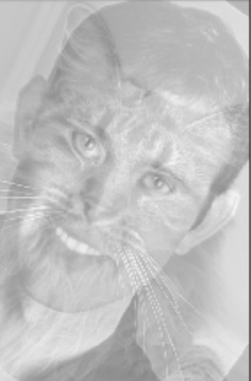
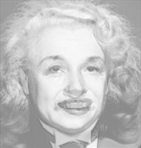
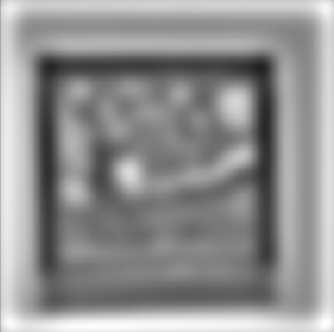
This case was a case where the images weren't properly combined because the images were aligned well."
Now, we create Guassian and Laplacian stacks. In order to create a Guassian stack for an image, we repeatedly apply a Gaussian filter(40x40, sigma=5) to the same image to create the levels of the stack. To create the levels of the Laplacian stack, you take the difference of each successive pair of levels in the Gaussian stack.
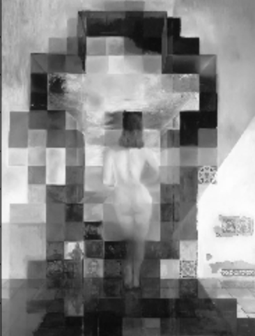


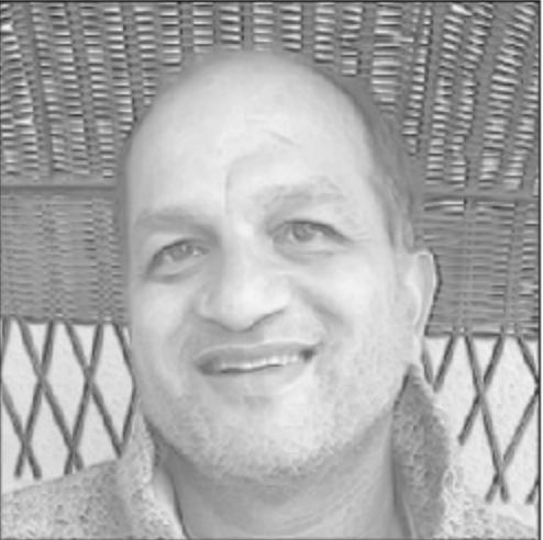
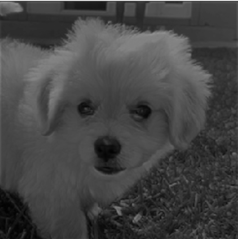
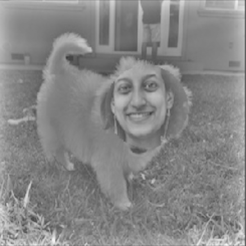
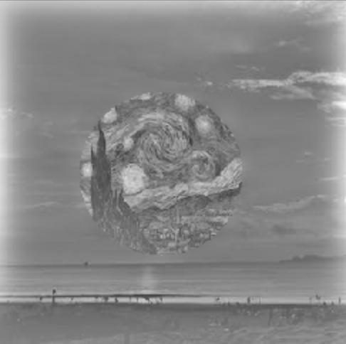
The goal of this part of the assignment is to blend two images seamlessly using a multi resolution blending. We use the Laplacian and Gaussian stacks that we created in the last part to achieve this. These stacks are used to break two images down into various frequency bands and then combine each band using a mask. This mask decides the weights for each image. For example, the circular mask is a 2d array with 1’s in a circle with a provided center position and radius. This is why a picture of my face appears on my dog in a circle in the hybrid image below. The resulting images are added together to create a hybrid blended image.


My favorite part of the project was definitely the last part, where we got to blend various images together. It was really cool to see all the different things you could do with various images. It was what people do with photoshop, except we were able to do it from scratch, which was really cool to do.
