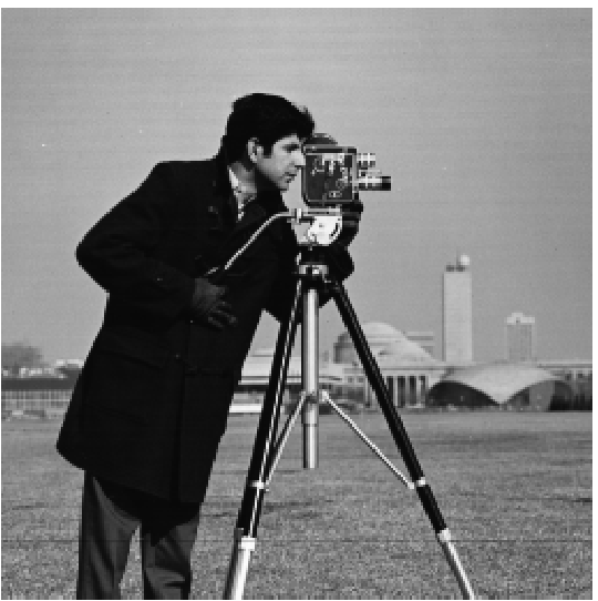
Introduction
The goal of this project was to understand different ways of using filters and frequencies on certain images and create awesome stuff.
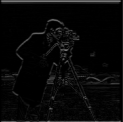
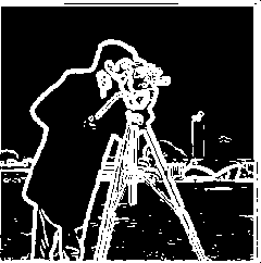
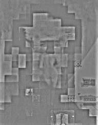
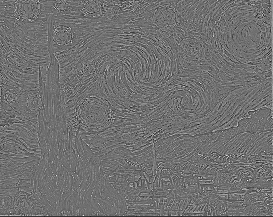
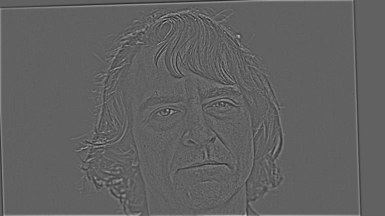
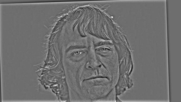
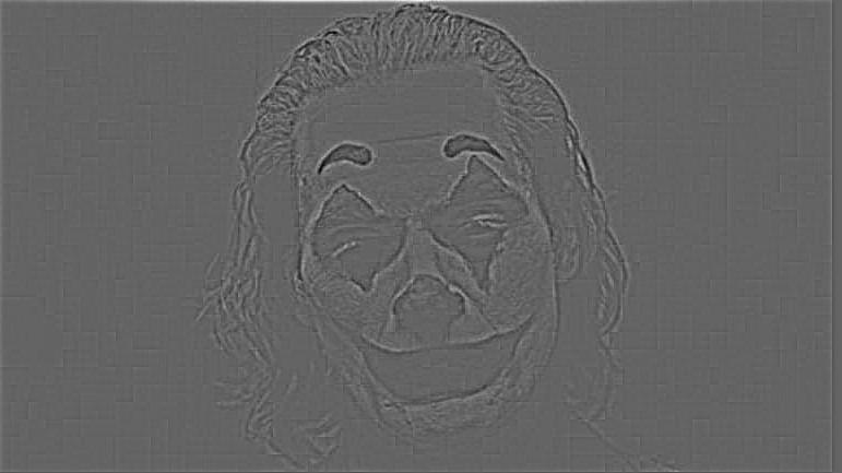
Part 1.1: Finite Difference Operator
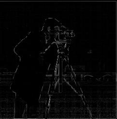
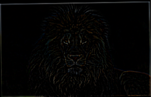
I convolved the cameraman image with d_x = [[1, -1], [0,0]] and d_y = d_x.T to get the partial derivatives of the image. Then I computed the gradient magnitude image by calculating the square root of the sum of the squares of the partial derivatives. Then I used Thresholding to only keeping pixels that were greater than a certain threshold (in this case, it was 0.13). This is how I created the binarized image of all the edges. The image, however, is slightly noisy, especially at the bottom.
|
|
|
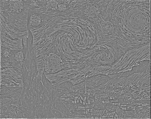
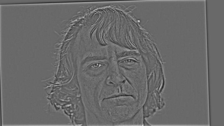
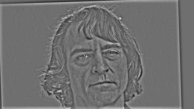
Part 1.2: Derivative of Gaussian (DoG) Filter
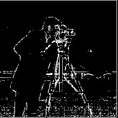
First way: I created a blurred version of the original image by convolving with a gaussian and repeated the procedure in the previous part. Then I moved on to find its edges by convolving the image with a 2D Gaussian kernel and got the gradient magnitude image. Then I used thresholding to binarize that image by only taking gradient magnitude pixel values that were greater than 0.016. The edges for this part were better then part 1.1 as we applied the gaussian and then got the edges.
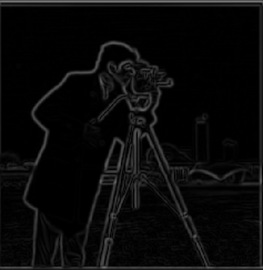
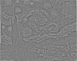
Second way: I found the Derivative of Gaussian on x axis (dx) and y axis (dy), and then applied them to the original unblurred image using convolution. As convolutions are commutative and associative we can either convolve our blurred image with our filters, or convolve the gaussian filters with the above filters before computing the gradient magnitude, both provided the same result.
|
|
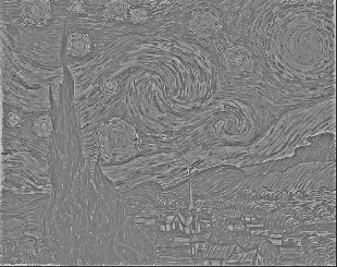
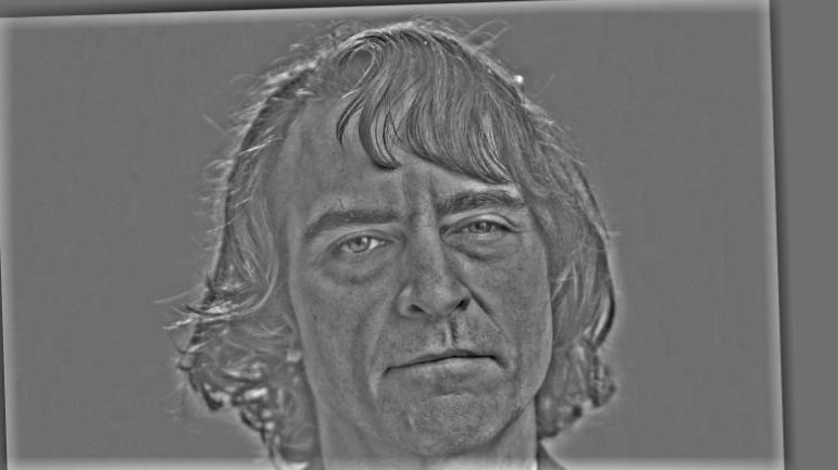
The binarized image for the first way s also displayed here:
|
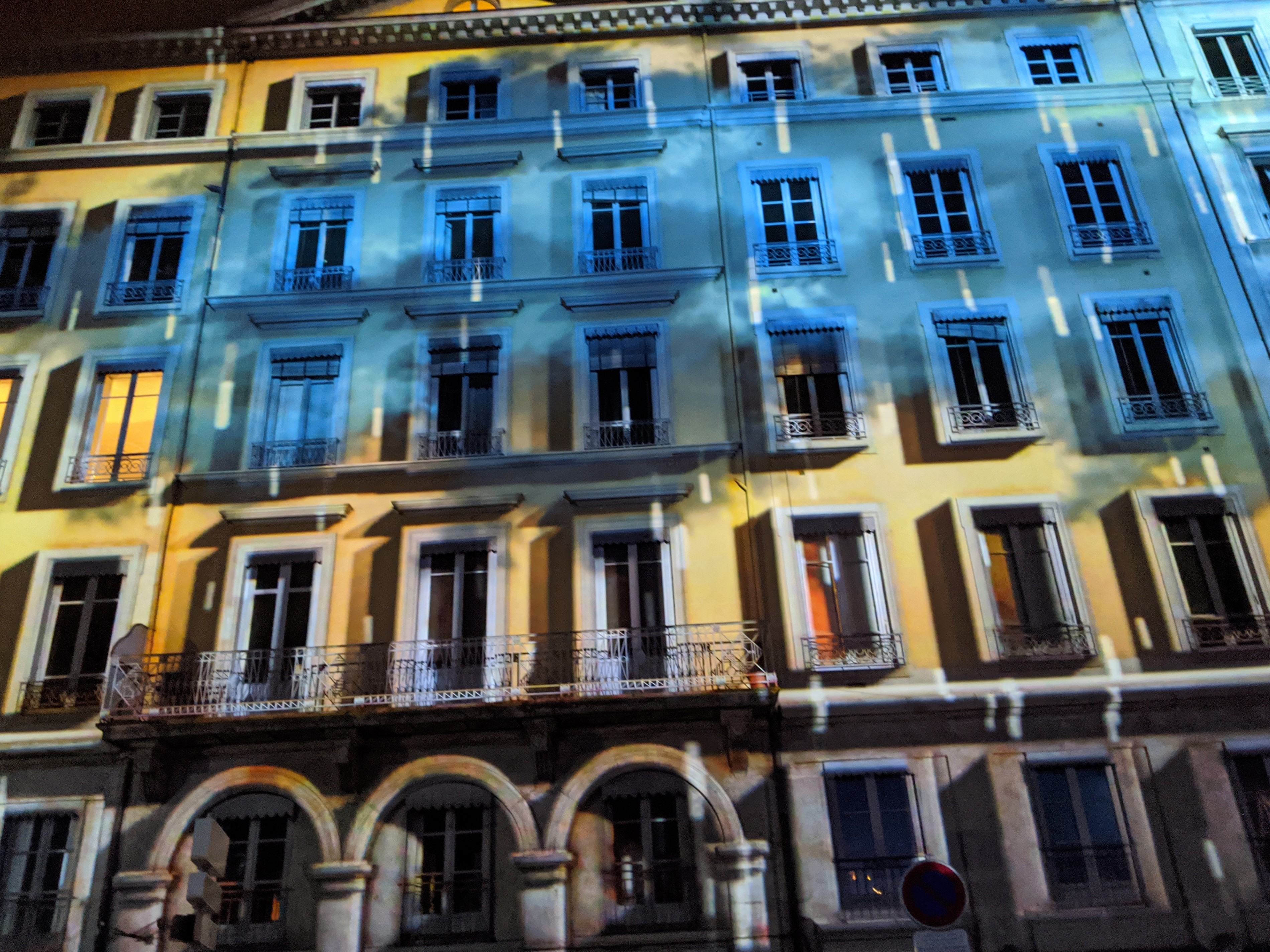
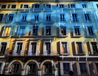
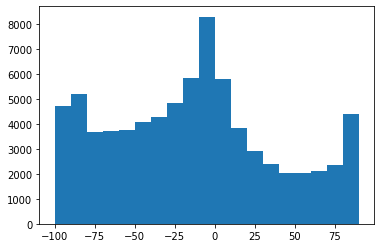
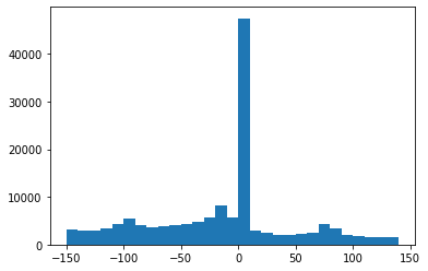
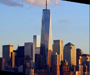
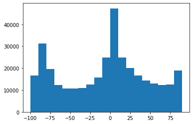
Part 1.3: Image Straightening
Facade
|
|
|
|
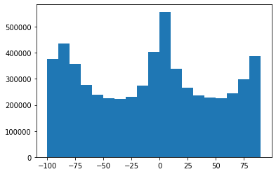
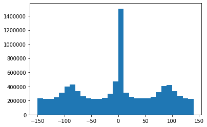
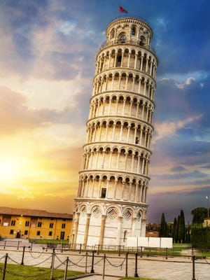
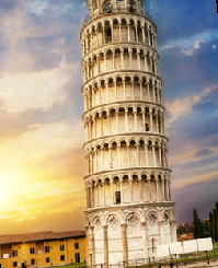
Leaning Tower of Pisa
|
|
|
|
Skyline

|
|
|
|
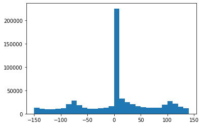
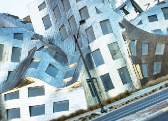
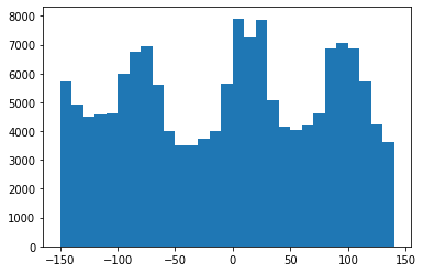
Curvy Building (Failure Case)
Here, the straightening function failed to straighten the image because the image contains curved edges that are hard to straighten.

|
|
|
|
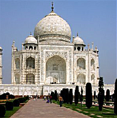
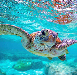
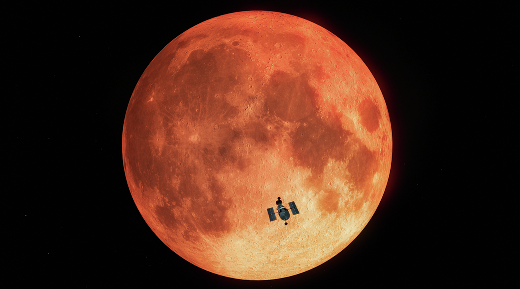
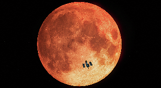
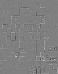
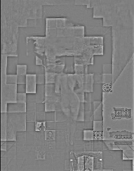
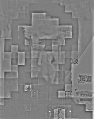
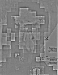
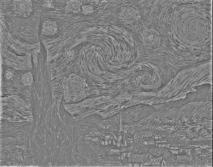
Part 2.1: Image "Sharpening"
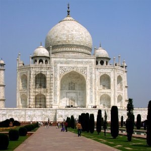
Taj Mahal
|
|
Sea Turtle

|
|
Moon
|
|
|
|
|
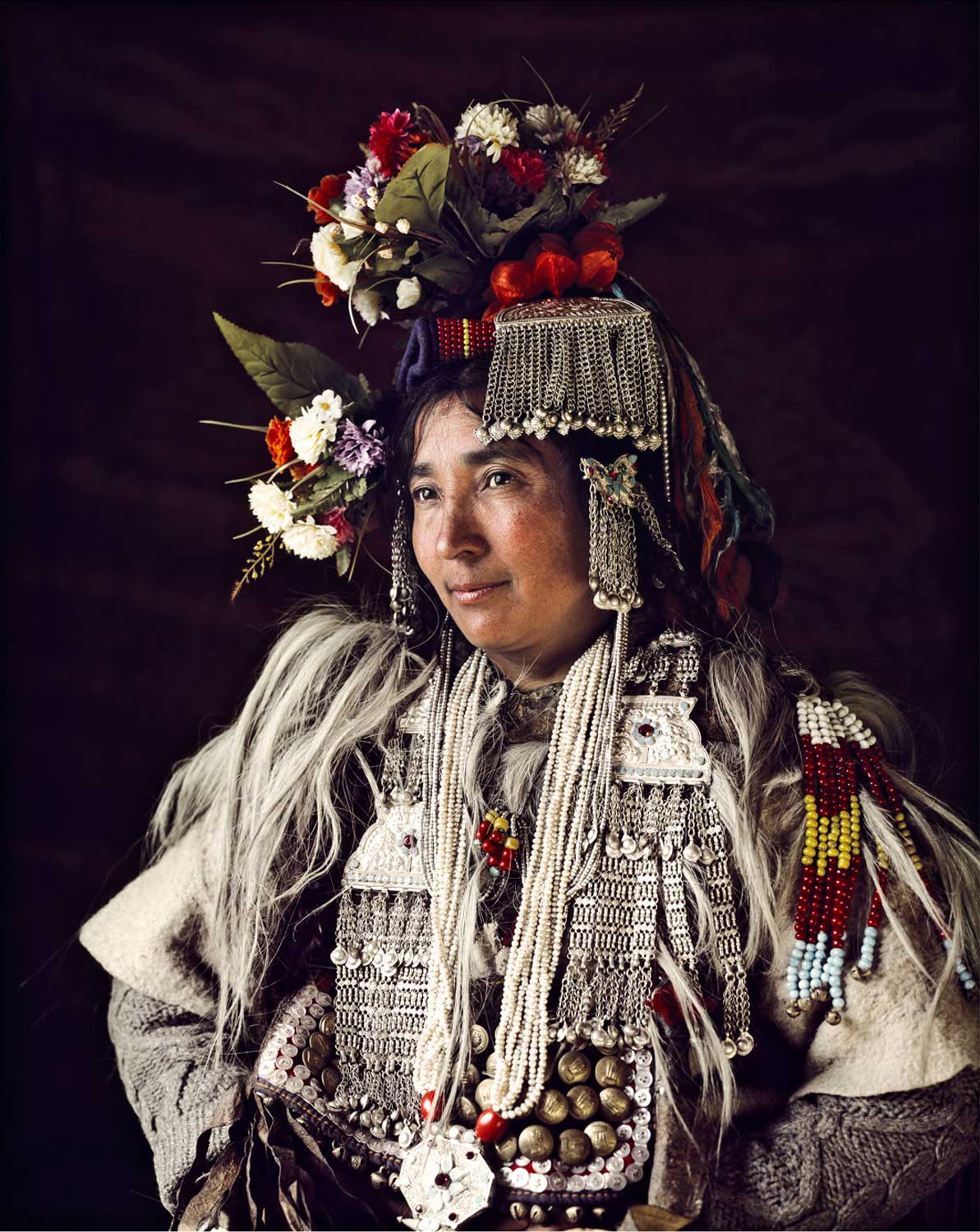
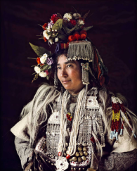
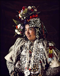
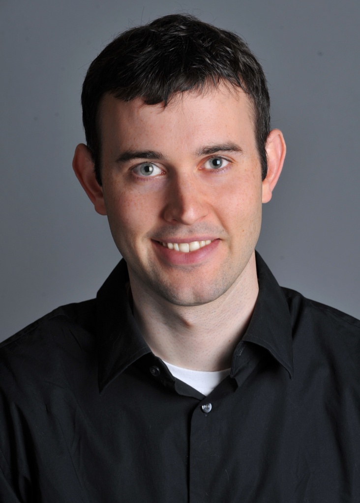
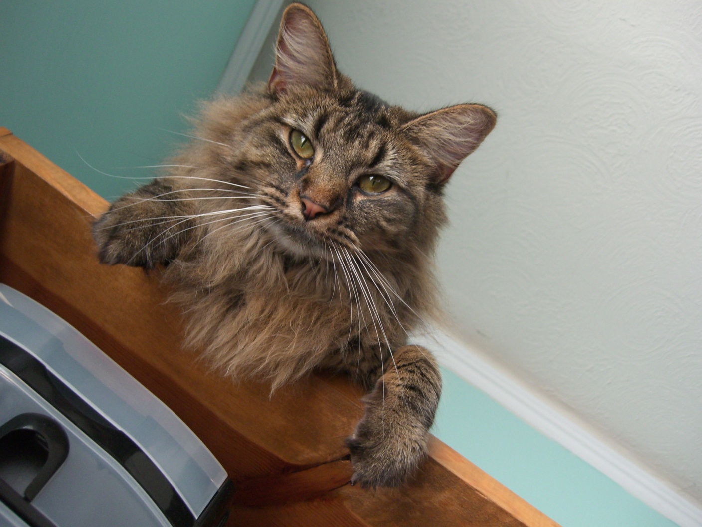
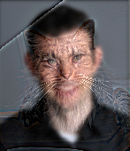
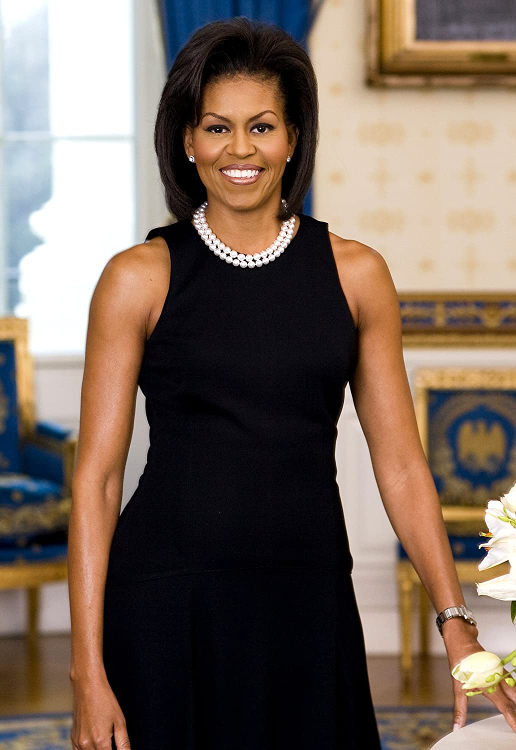
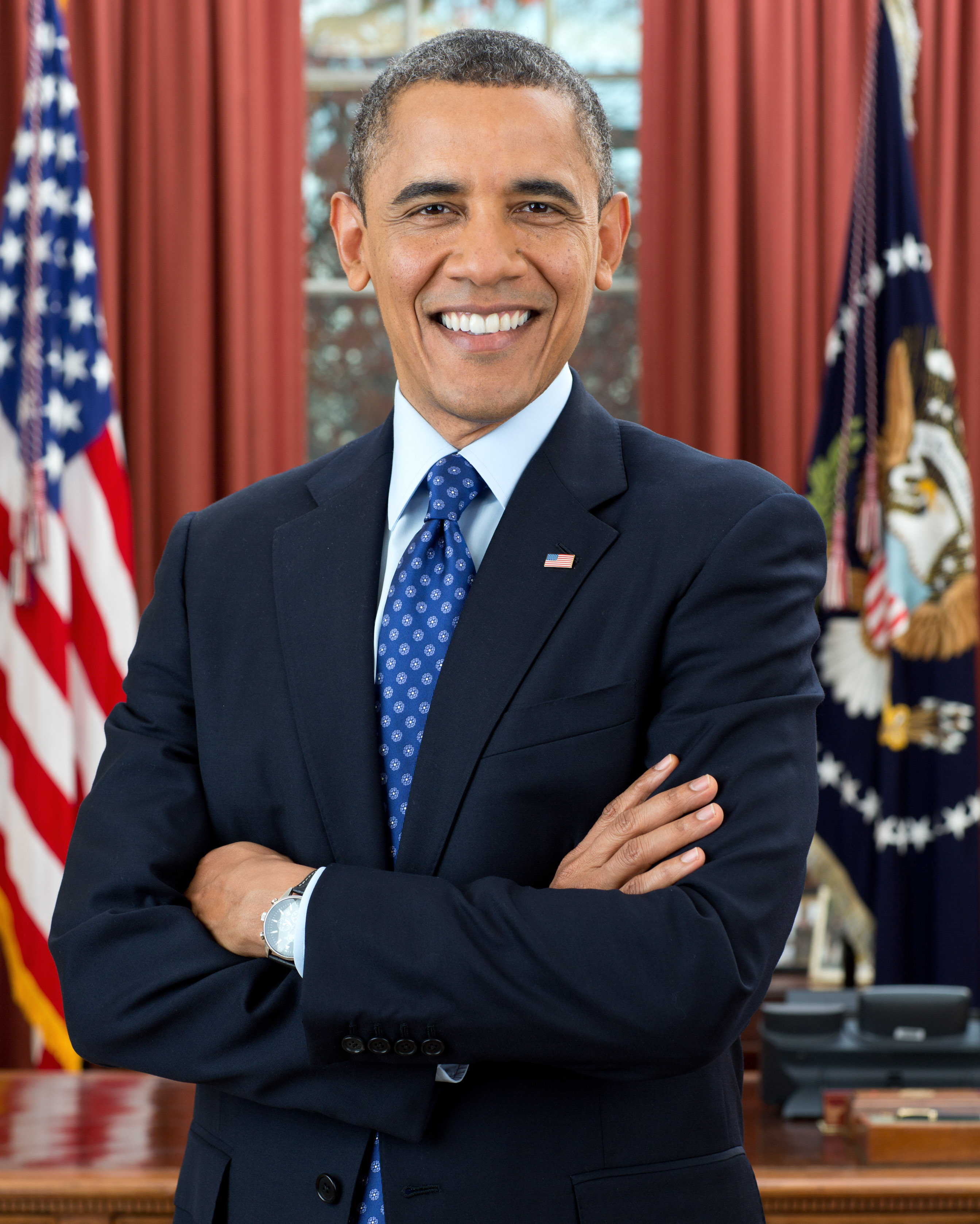
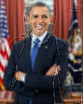
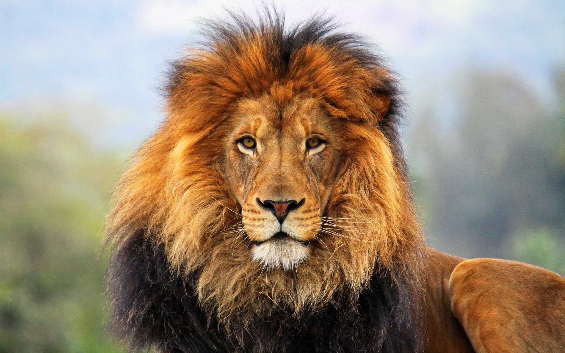
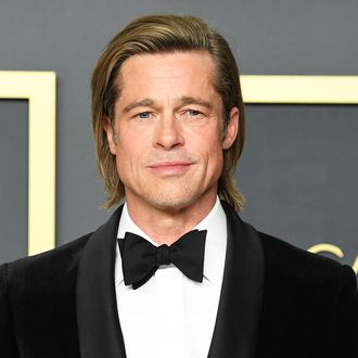
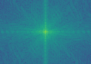
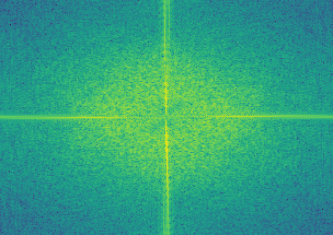
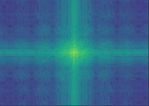
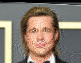
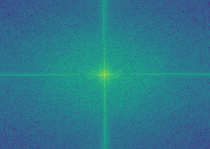
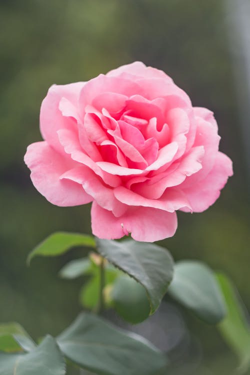
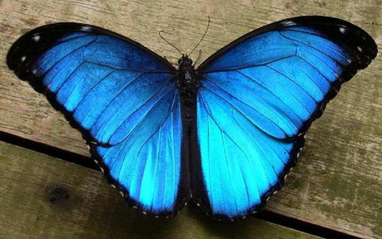
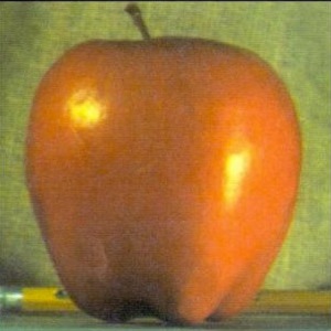
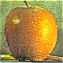
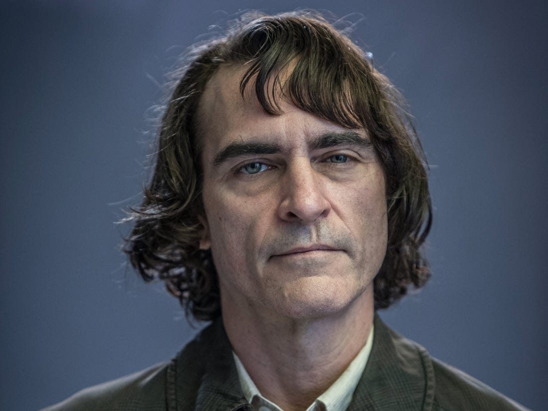
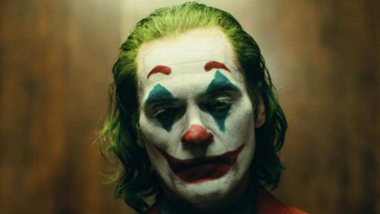
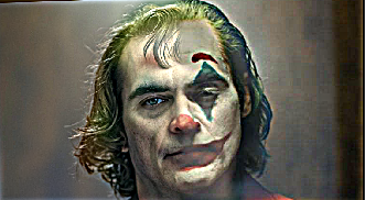
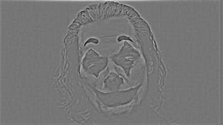
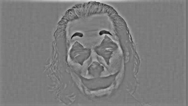
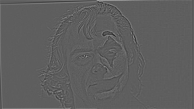
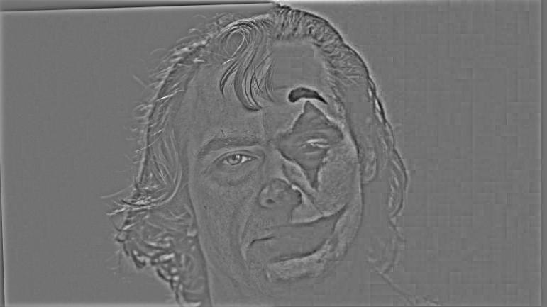
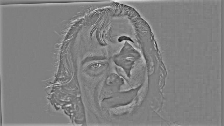
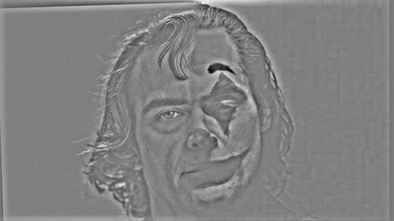
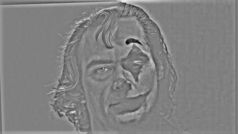
Part 2.2: Hybrid Images with Bells and Whistles
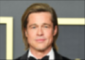
I created these hybrid images by ,first, aligning them based on the postion of the eyes, and then adding the high frequency image of one to the low frequency image of the other. These hybrid images were created after adding color by auto contrasting from the beginning.
|
|
|
|
|
|
|
|
|
|
|
|
|
|
|
|
|
|
|
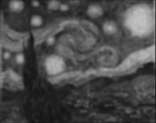
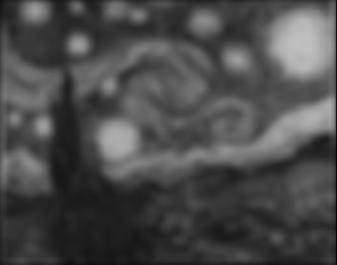
Part 2.3: Gaussian and Laplacian Stacks
As mentioned in the project spec, I created a Gaussian and Laplacian stack by taking a normal image and iterating through 5 levels without downsampling it and applying Gaussian and Laplacian (original image - Gaussian blur image) filter of sigma = [2,4,8,16,32] to the image.
|
|
|
|
|
|
|
|
|
|
|
|
|
|

|
|
|

|

|
|
|
|
|
|
|
|
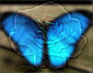
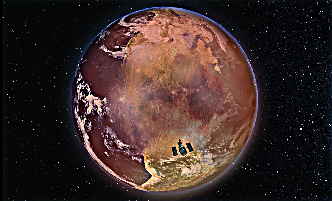
Part 2.4: Multiresolution Blending
I used the techniques shown in Burt and Adelson's 1983 paper on Multiresolution Spline to create a function that leverages Gaussian and Laplacian stacks. This function takes in 2 images and outputs the blended image (by summing the Laplacian stacks and adding the last gaussian stack to it).
|

|
|

|
|
|
|
|
|
|
|
|
|
|
|

|

|
|
|
|
|
|
|
|
|
|

|
Key Takeaways
The most interesting part about this project was learning how everything comes together at the end after estimating derivative to using gaussian blur technique and then to creating amazing masked/blended images.