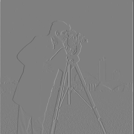
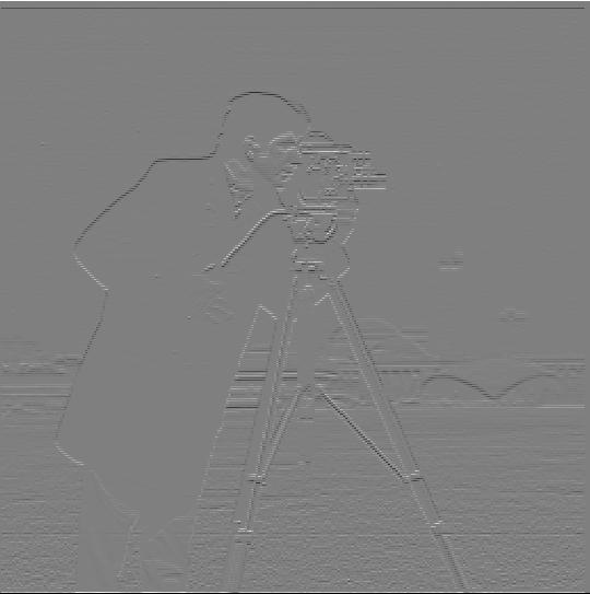
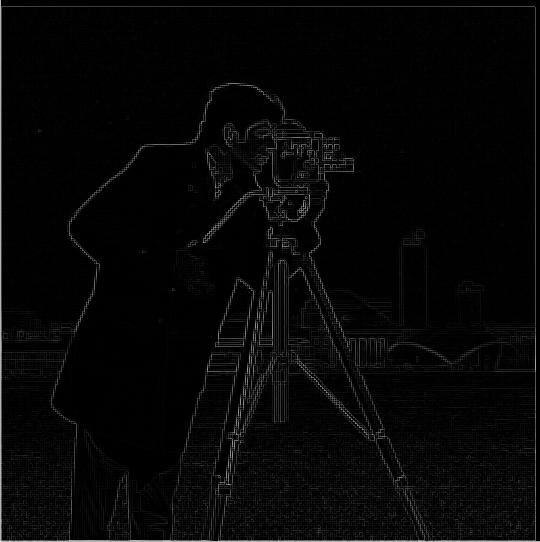
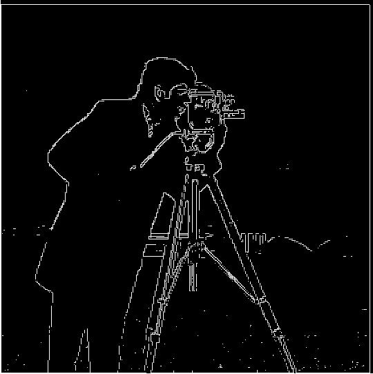
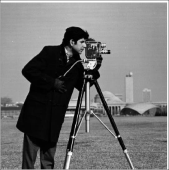
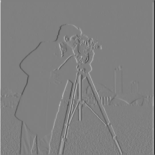
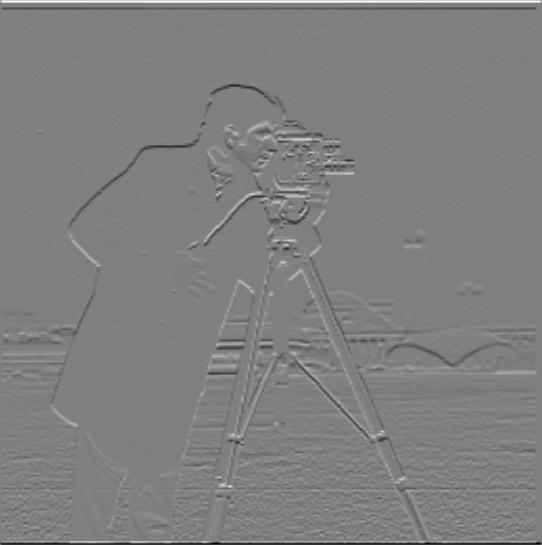
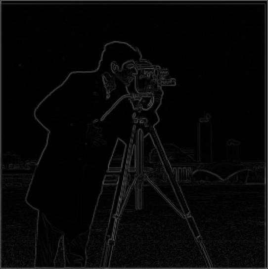
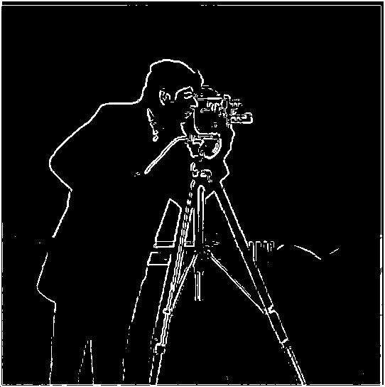
Partial derivative in xPartial derivative in yGradient magnitudeEdges (threshold of 0.25)
To compute the gradient magnitude, we sum the element-wise squares of the two partial derivative images, then take the
square root of the result. In pseudocode, gradient_magnitude = sqrt((partial_x ** 2) + (partial_y ** 2)).
1.2
Filtered cameraman Partial derivative in x, after filteringPartial derivative in y, after filteringGradient magnitude, after filteringEdges, after filtering (threshold of 0.13)
After filtering, we get much better results. In particular, the partial derivatives are relatively
stronger around the cameraman's body, which makes it easier to separate the true edges from
the noise using a threshold. We can see that despite having a lower threshold, the edge image
is now much clearer, more accurate, and less noisy.
DoG filter in xDoG filter in yGradient magnitude, using DoGEdges, using DoG (threshold of 0.13)
We can see that DoG results in the same output images.
1.3
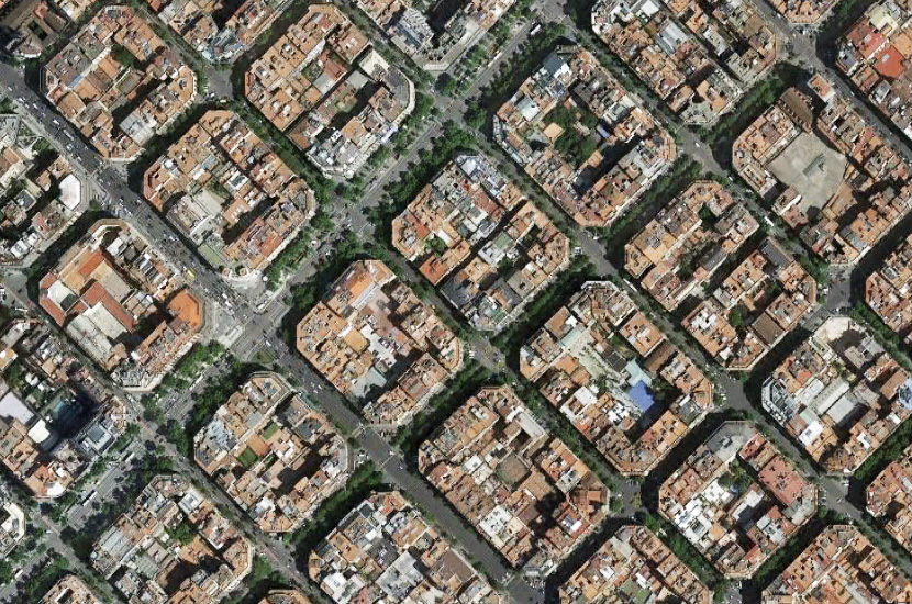
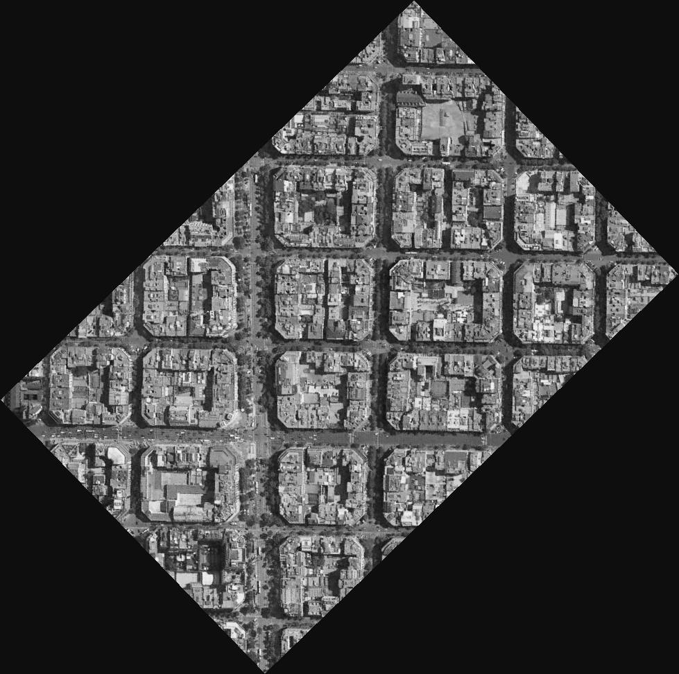
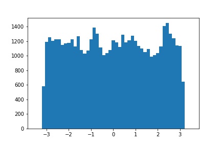
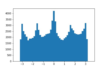
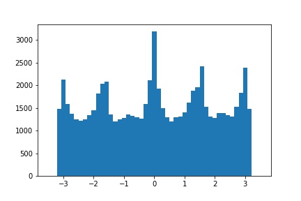
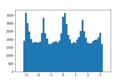
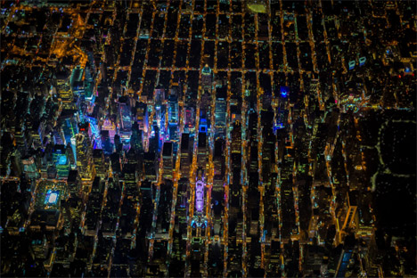
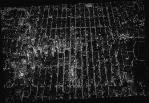
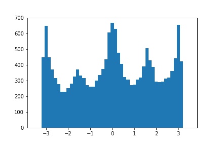
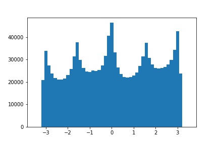
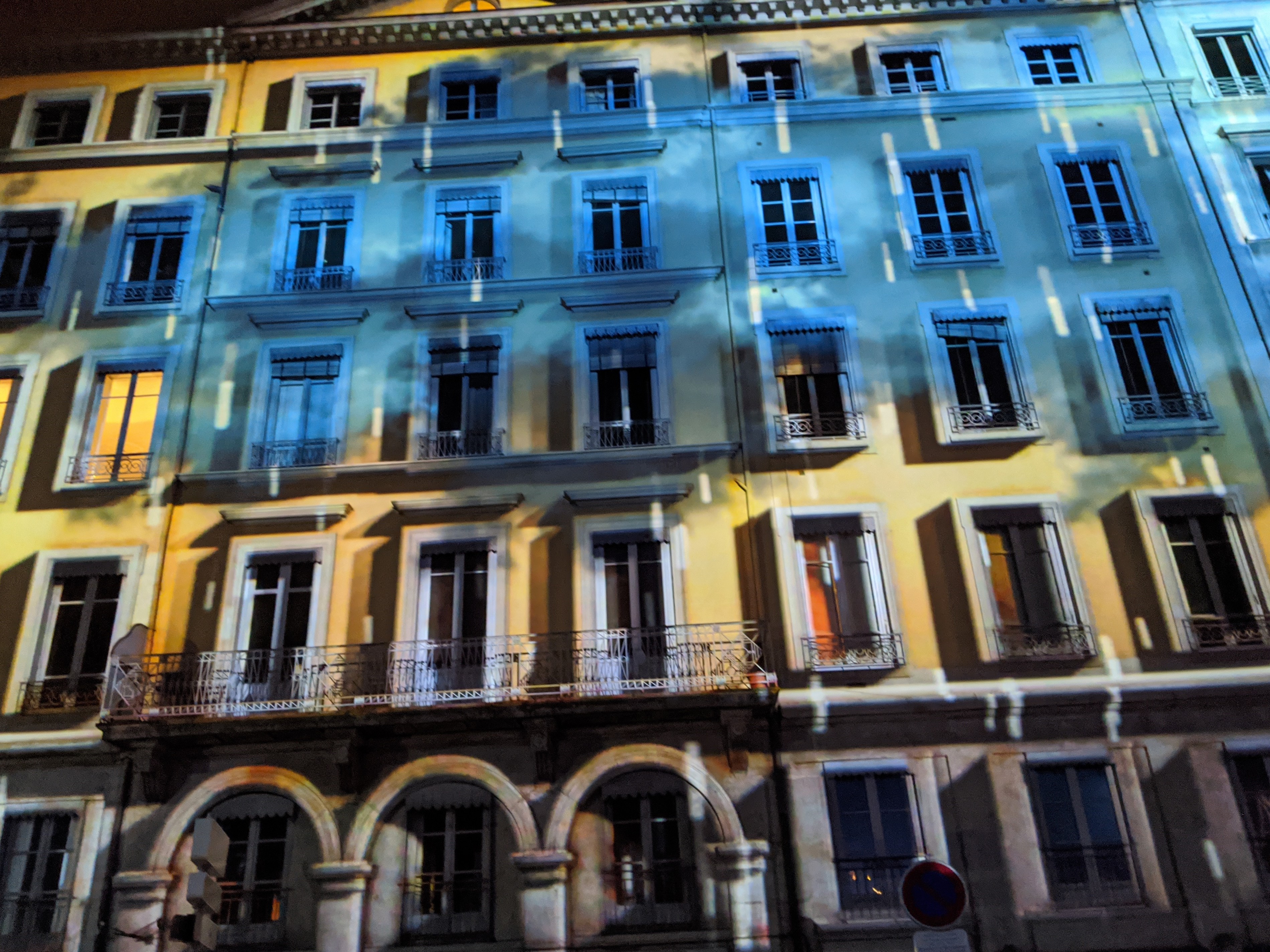
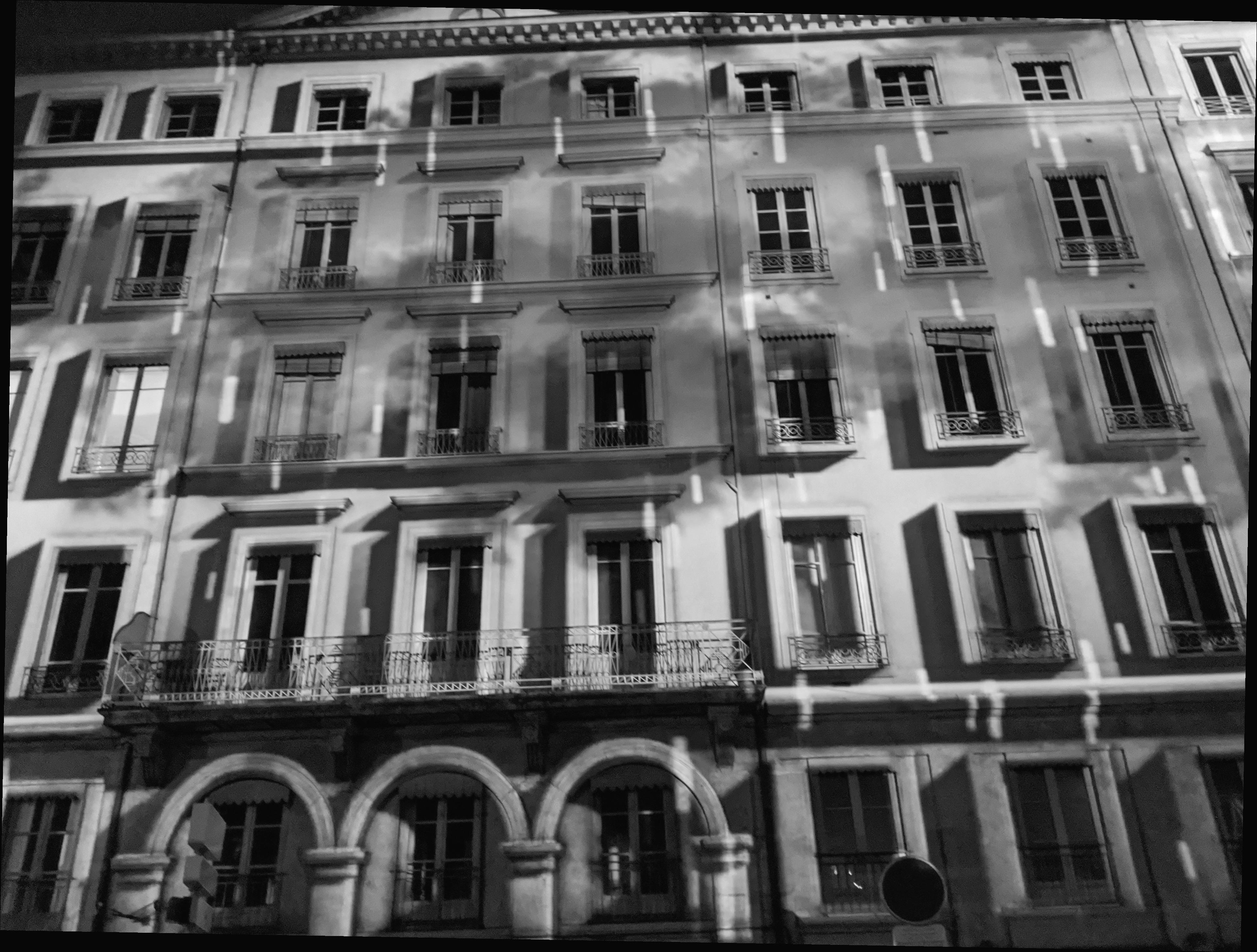
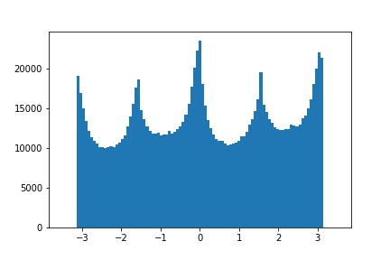
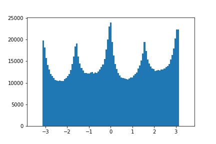
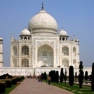
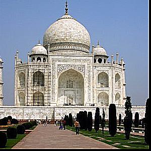
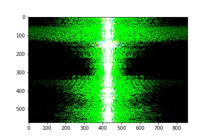
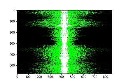
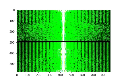
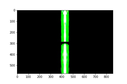
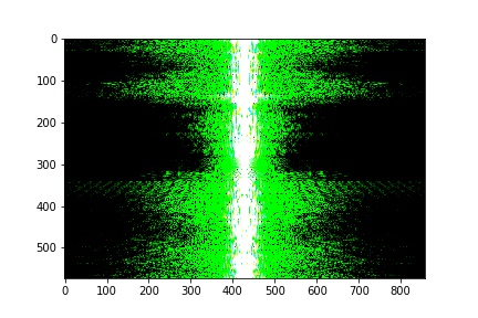
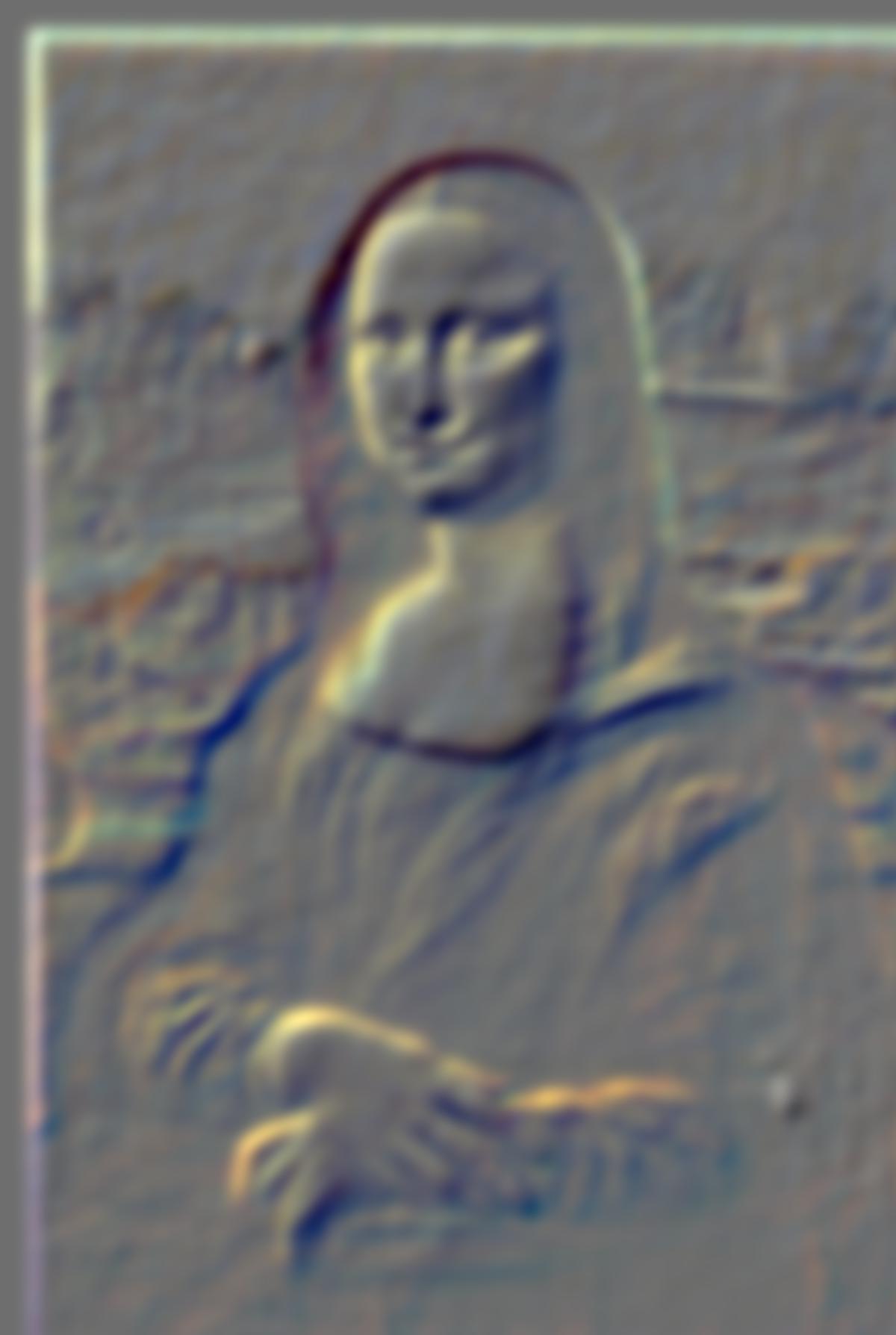
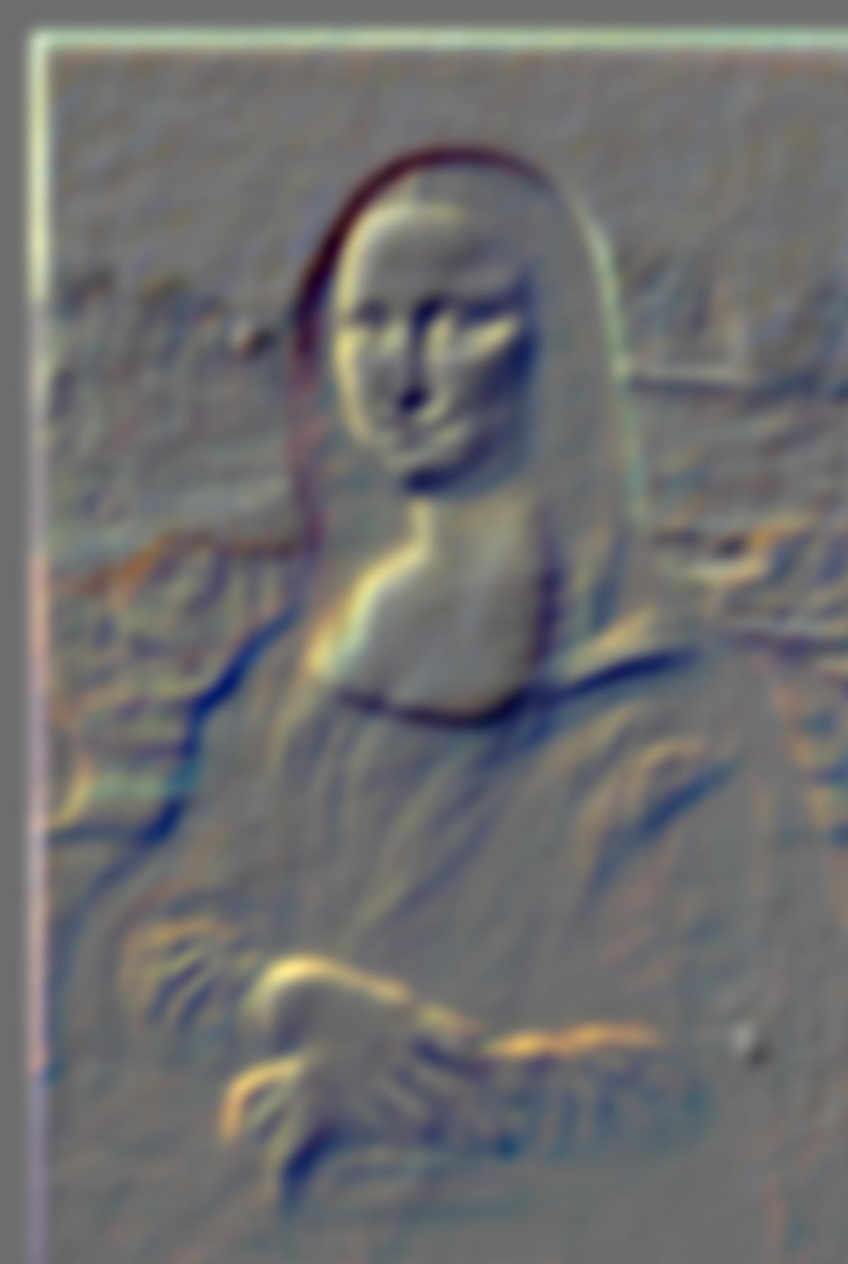
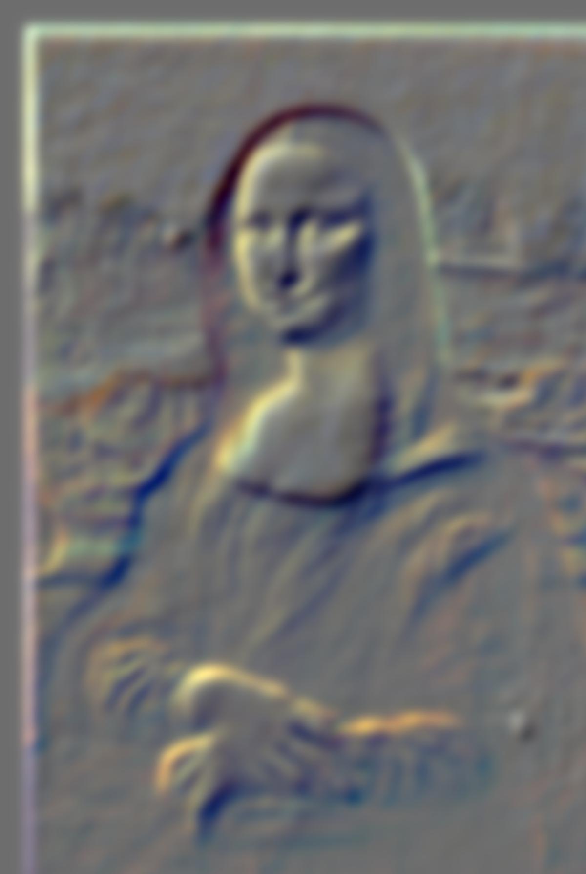
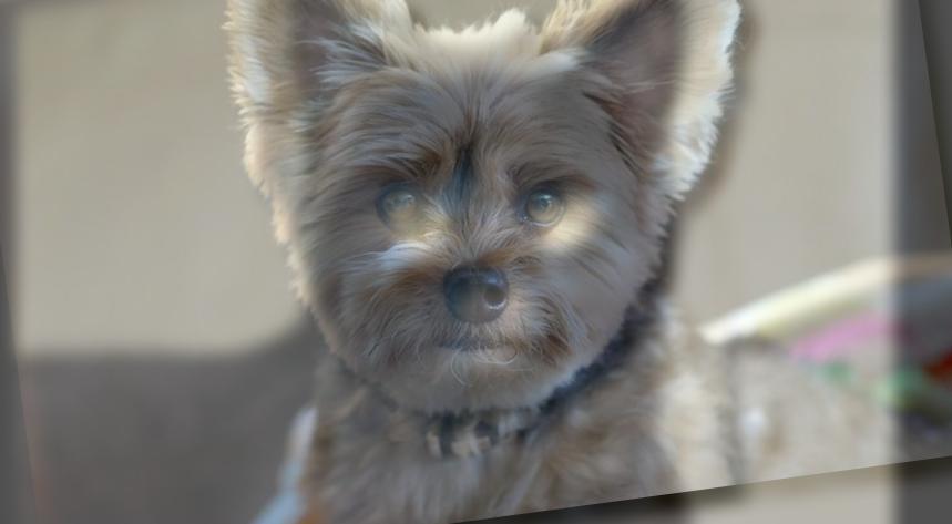
For test images, the order is original, rotated, original histogram, rotated histogram.
Barcelona:
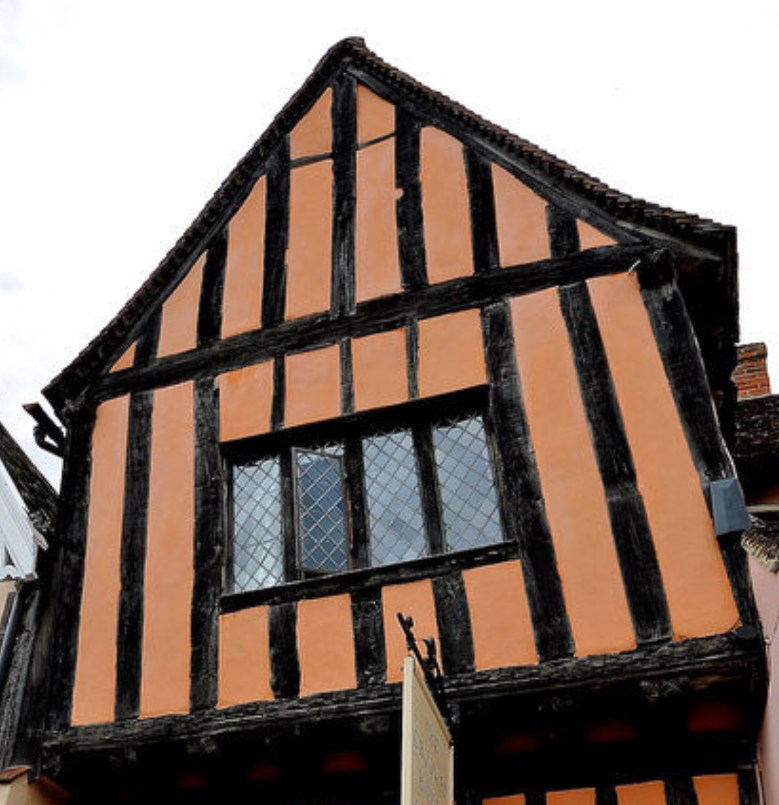
House:
This is probably the failure case, since the algorithm overcorrects.