Overview

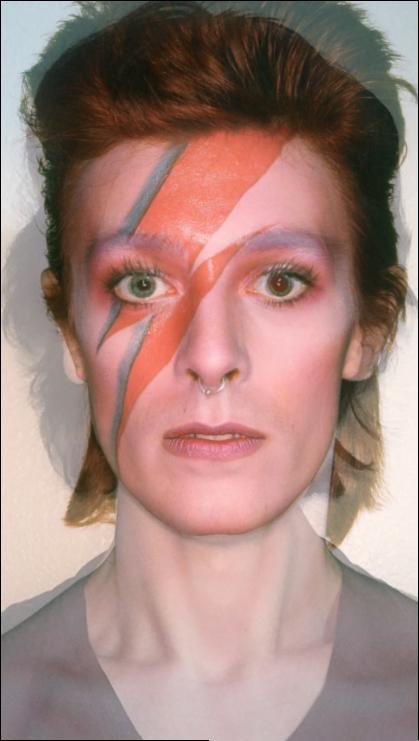
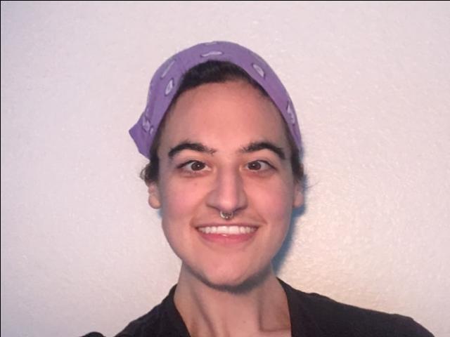
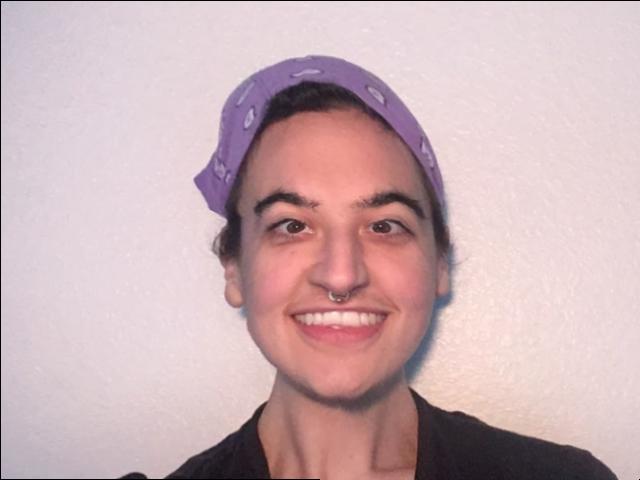
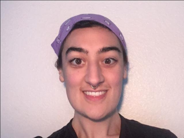
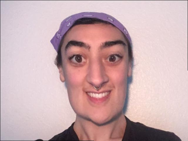
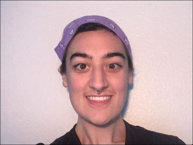
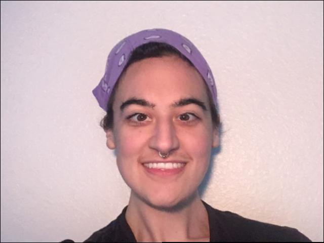
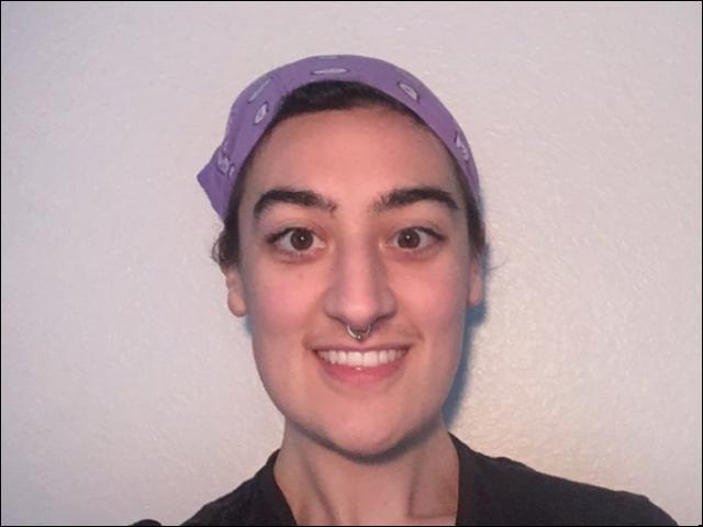
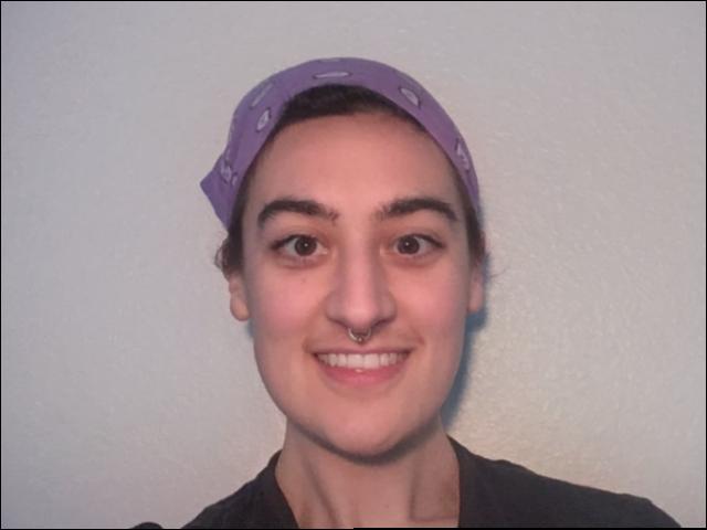
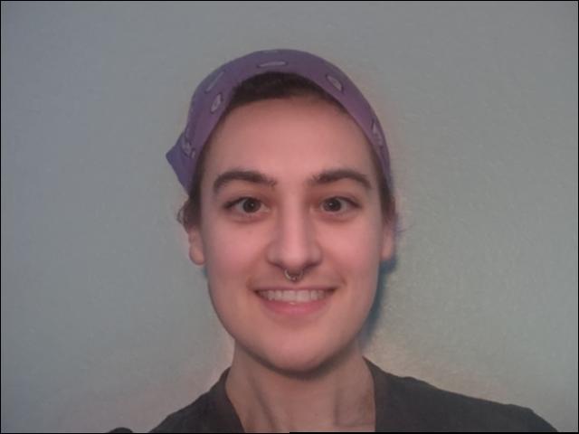
Two images can be morphed together in a convincing way if you choose your correspondences and starting images wisely. I went through a few different images/test points until I found a nice head-on image to use of myself and to warp to. I found that aligning the images made for better morphing and helped me get around the fact that I can never truly replicate the studio setup of a photograph I found online. That said, I tried to take pictures that were close as I could manage to begin with, then used align_images to make up for whatever minor differences remained and ensure the images would be the same size.

Defining correspondences

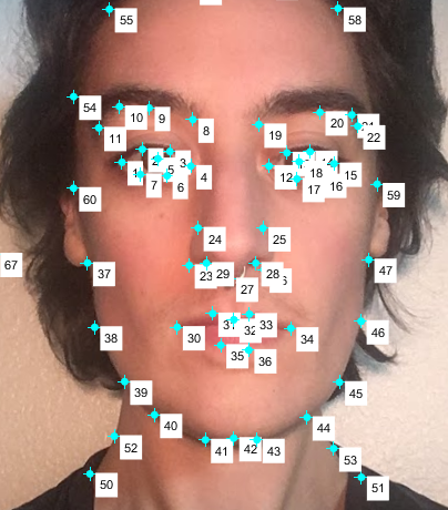
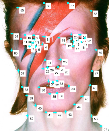
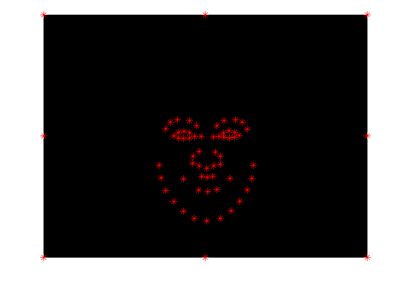
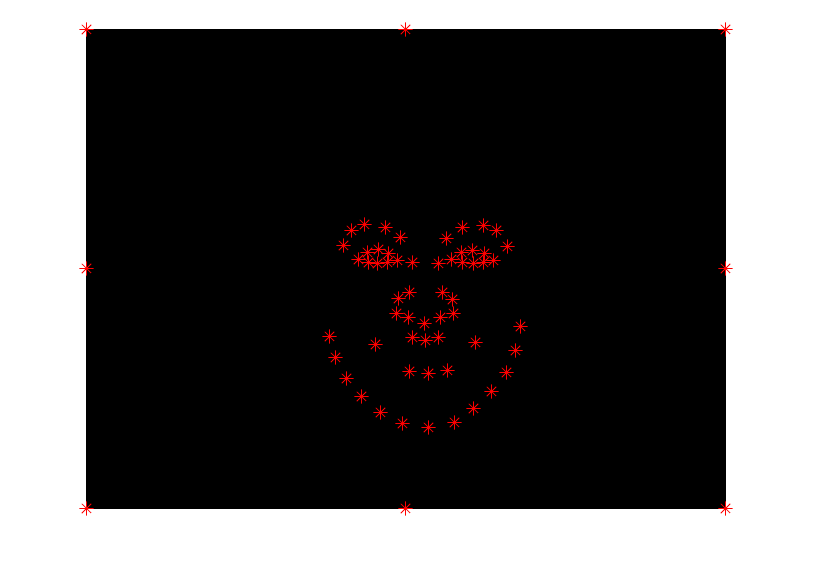
I followed the example from the Danes dataset and chose correspondences around the mouth, nose, eyes, and chin first. Then, I chose some extras around the neck, forehead, and cheeks to make the morph more fluid.

As you can see from the pictures, I used quite a few. After using the cpselect tool in matlab to make all these correspondences, I also wrote a function that would apply some around the four corners and midpoints between them to act as 'anchor' points.

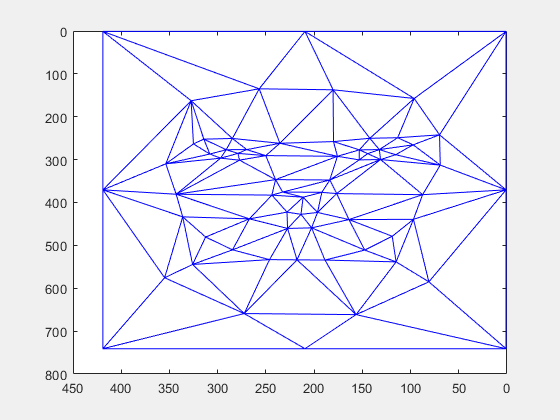
After getting the correspondences, I averaged them to get the average points between the two images. Using this average, I made a triangulation using the delaunay function.

It looks a little strange without the midway face for reference, so let's get started on that:

To create the midway face, I implemented computeAffine. I did this by using the triangulation to get the vertices of the triangles in the moving image and the fixed image. With these vertices, I found the affine transformation per triangle by using the standard basis as an 'in between' transformation for the two images. For instance, say I want to go from image A to image B, and I have all of the triangle vertices. I can find the affine transformation from the standard basis to Image A by setting one of the vertices to be the new 'origin', and subtracting that vertex from the others. I fill the bottom row with 0, 0, 1 to represent the two legs of the triangles as vectors and the shared vertex as the new origin. I do the same for standard basis->image B. Then, I can take the inverse of the first transformation and combine them to get a transformation that can take a triangle in image A -> std basis -> image B.

Now, I iterate through all triangles in the triangulation and apply each triangle's transform to all of the pixels in that triangle. How to get the pixels? I used a mask to isolate them and get the (x,y) locations of pixels inside the triangle in the 'destination image'. Then, I used the inverse affine transform at that triangle to go backwards into image A or B and fill that location with the color at the pixel's old location in the source images. I used interp2d to accomplish this. For the midway image, I used the average point location as the 'destination points', and image A/B as the 'source points' and 'source image'. I transformed both of their points to the average points and interpolated the colors from the source image. Finally, I averaged those interpolations to get the midway color. Here is the result:

The morph sequence

Now that the midway is done, time for a full morph. To do the morph, I pretty much did what I did above, but instead of weighing things to .5 as I did with an average, I used a sliding scale from [0,1] to weigh the shape transforms/color transforms gradually from image A to image B, then wrote them all together in a gif.

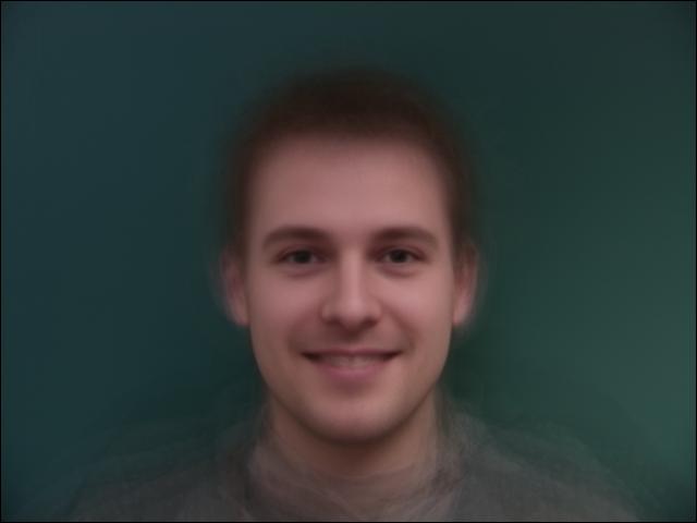
"Mean Face" of a population

For this task, I chose the Danes dataset since their keypoints came with the data. I imported the front facing happy and neutral images for both men and women in the dataset. To get the average face for the Danes, I iterated through all of their keypoints and averaged them (I did this for men, women, and the entire population). Once I had the average shape, I warped them all to that shape using computeAffine and similar interpolation procedures as above. I also took the liberty of adding some anchor points to make the images a little more interesting.

The points weren't too different from one submean to the other, so I didn't save any of the other plots. I randomly chose 3 faces from each submean of smiling men and women to warp to the average. Here are some of those:

And now, for the actual average faces:

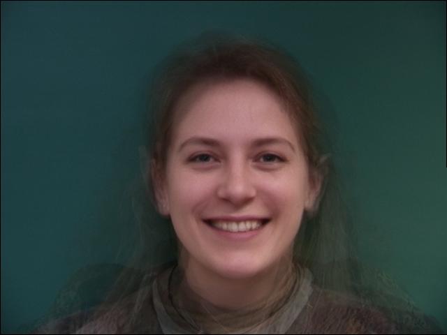
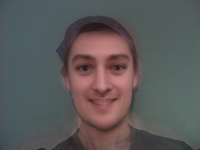
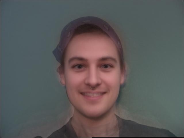
A prelude to caricatures-- here is my face warped to the average, and the average warped to me.

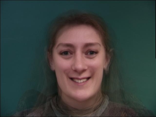
Caricatures

We can make a caricature by subtracting what makes us different from a mean and adding that difference back to the original image, scaled by some modifier. My caricatures were created by subtracting the mean shape from my face's shape, then adding that difference back in scaled by some alpha between .1 and .99. I found that if I used alphas greater than one, the image was severely distorted and while it was a caricature, it was almost too extreme to really get anything meaningful from it.

As you can see, the things about my face that are different from the mean face of Danish women get more and more exaggerated as you add in larger amounts of the difference from the mean.

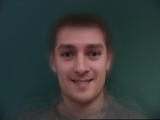
A required bell and whistle - gender shift

I thought it might be interesting to see how my face might look if I amped up the things it has in common with the average male face. To do this, I pretty much did the reverse of a caricature from earlier-- instead of adding the difference of my face from the mean, I subtracted it to make my face less like mine and more like the mean.

Here are the shape shifts...

Color shifts...

Now for everything:

One extra bell and whistle - class video

link: https://tinyurl.com/194-26-classvid

Citation for Danes dataset

M. B. Stegmann, B. K. Ersbøll, and R. Larsen. FAME – a flexible appearance modellingenvironment. IEEE Trans. on Medical Imaging, 22(10):1319–1331, 2003
@ARTICLE{Stegmann2003tmi,
author = "M. B. Stegmann and B. K. Ersb{\o}ll and R. Larsen",
title = "{FAME} -- A Flexible Appearance Modelling Environment",
year = "2003",
pages = "1319-1331",
journal = "IEEE Trans. on Medical Imaging",
volume = "22",
number = "10",
publisher = "IEEE"