It turns out that human faces, unlike most things share a common structure across our population. As a result, this makes it relatively easy to morph faces
into each other using warps. By applying some clever forms of linear algebra, we can not only morph the color of our faces, but we can also morph the structure of our faces.
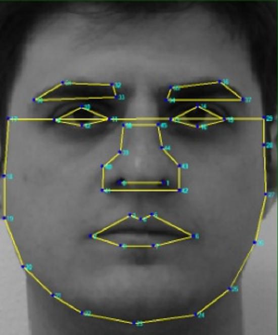
To do this, we need to encode basic structure about our images in the form of facial keypoints . These are corresponding points between two faces that are used to identify the
facial features of the two people, for example the top of the lip, or the top most point on the left eyebrow. An example of a set of 46 keypoints can be found below:
As such, for this project, we wrote code to capture some number of keypoints and save them as ".npy" files.
Computing the Midway Face
In order to compute the midway face, we can take advatnage of both the gemetric structure defined by our keypoints and the pixel colors in our image. To do this,
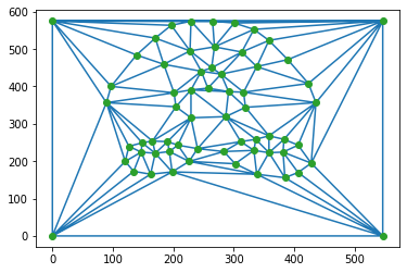
we compute a triangulation on top of our keypoints called the "Delaunay Triangulation". This is a special triangulation that is related to Vornoi Diagrams and can be
easily constructed given a set of keypoints.
We first average our keypoint positions on both faces and compute the triangulation on this new average keypoint set. This will ensure that the triangulation will be
non-degenerate and well-posed for both images.
We can see what an example Delaunay Triangulation looks like here:
We now have triangles which we can use in our average image. For each triangle, we compute the set of pixels inside that triangle. We then compute the inverse affine transformation from the average triangle
to the corresponding triangle on each face. For each point in a given triangle, we apply this transformation to find its corresponding pixel in each image. If the pixel is not a perfect integer, we simply average
its surrounding pixels to determine its color. From here, we take a weighted average between the start and end image to determine the final color of the pixel.
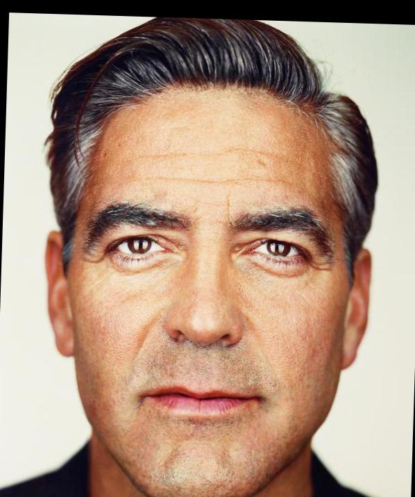
Here we see George Cloony and the Author of this Article and their mid-way face.
Morphing Faces into Each Other
In the last section we discussed computing the average face. However, we can also interpolate between faces continuously! To see this, we need only modify the algorithm used in the last
section.
We did two things:
We found the average shape by computing the average keypoint. Instead, we can linearly interpolate between the two keypoints by using a convex combination of the keypoints!
We found the color of the pixels by computing an average between the corresponding pixels in one image vs the other. We can similarly do an interpolated average by doing a convex combination of the two pixel values!
Essentially, we interpolate between shape and color separately, having one parameter as to how much of one face's shape we want, and another determining how much of one's color we want. Doing this over and over, we end up with the following video:
Here is another video that the author did with his classmates (Bells and Whistles)!
The Average Face of a Population
We now move on to applying this type of averaging / morphint to multiple images. In fact, we can do such a thing with an entire population!
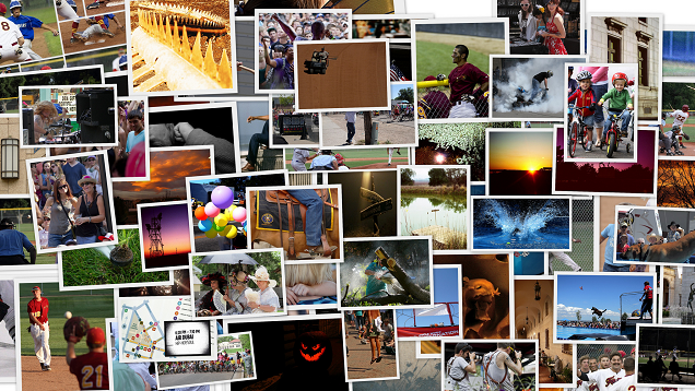
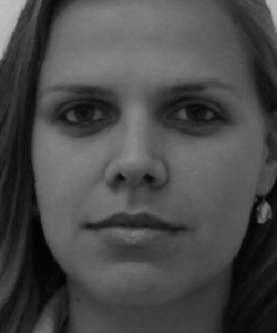
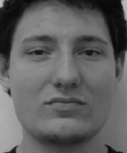
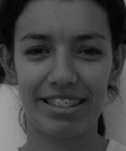
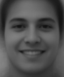
We used this database in order to compute the average smiling and average serious/frowning faces. Some example images from this dataset are:
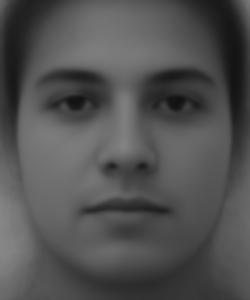
Similar to the mid-way face computation from the previous section, we can weight each image in this set equally and compute the "average" face over this entire population. We simply
need to set each person's shape and color weight to be equal across the population. Doing so yields the following results for both the smiling and serious faces.
What is amazing, is that the face is perfectly symmetrical and gender neutral, yet the smile and frown features are distinctly present in their respective images. Here are some image morphs of these images into
the final dataset.
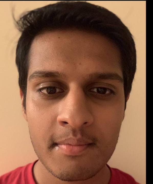
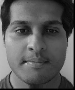
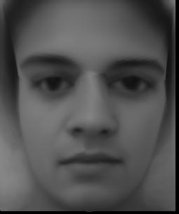
Finally, we can go back and look at a completely different image, and understand how it gets mapped into this dataset. In this case, we will use the author's image. Below is the author's image, the author's image with the
average face's geometry, and the average face with the author's geometry. In this case, since the author is serious/frowning, we say the population is the frowning face.
Caricatures and Feature Transformations
Caricatures
Finally, we can use our technique that we have developed to do caricatures and feature transformations. Caricatures are just natural extentions of what makes us
not average. Thus if we extrapolate the average face through an existing face, we should be able to determine what extrapolations make the face unique. We produce a caricature of the author's face below:
Feature Transformations (Bells and Whistles)
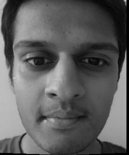
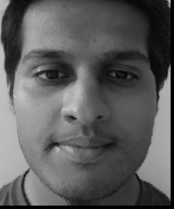
Lastly, we can interpolate between an average "smiling" population and the author's face in order to get the author to smile! In this case, we want to keep the
geometry of the average face, but the color of the author, so we don't interpolate on color, just on the geometry. Doing so yields: