We used the IMM dataset for nose keypoint detection. In order to do this, we needed to first write a pytorch dataloader to load the images. This is done by
reading the correct file and transforming it into a PIL image. We are lucky that pytorch's Dataset and Dataloader class abstract away most of the complexity surrounding
doing these things.
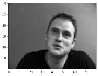
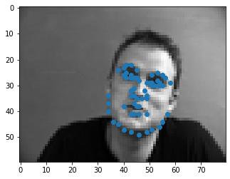
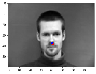
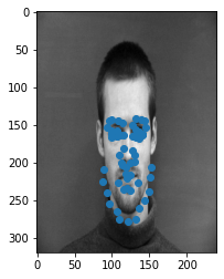
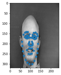
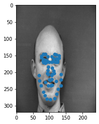
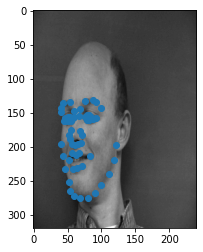
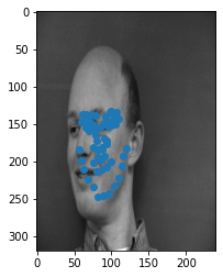
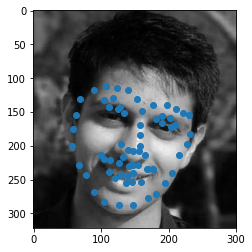
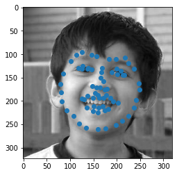
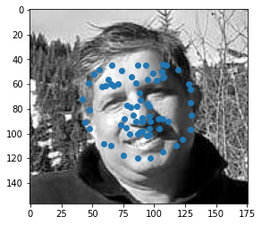
Here are some example images from the dataset. The dot nearest to the nose represents the nose keypoint!
In order to detect the keypoints, we have to use a convolutional neural network (CNN) to read in the image and output a prediction. We decided to use the following architecture for our neural network.
Note: Each convolutional layer is 1 convolutiona layer followed by a ReLU and then a 2D Max Pool. The first fully connected layer also has a ReLu activation. All convolutional weights are initalized
with kaiming uniform weights. The fully connected layers have xaiver uniform weights. Biases were initalized to 0.
We trained this network on images of size 80 X 60 for 25 Epochs. There were 192 images in our training set and 48 images in our test set. Note this is a pretty severe lack of data for a CNN.
This CNN produced somewhat mixed results. We believe this is primarily because of the severe lack of data available. If we had applied data augmentations or simply had more images this would have likely greatly improved
our predictability. In addition, had the images been bigger or the neural network had more channels, it is likely our network would have performed stronger.
My ultimate theory as to why these are failures are that the point is most closely associated with the brightest pixel on the screen. In most of these images, this brightest
point lies near the nose since that is often what is most well illuminated. I believe that this network is not taking into account the rest of the image and so it is only detecting the brightest pixel.
Part 2: Full Facial Keypoint Detection
We now aim to enhance our previous network into a network that can detect 58 keypoints on various parts of the image!
Adding Data Augmentations
As we saw in the previous section, our network does not perform well if we don't have that much data. We remedy this in two ways:
- We increase the amount of data per image by increasing the input size to a 320 X 240 image.
- We apply the following data augmentations to add more data:
- Rotation between [-15, 15] degrees
- Translation within 25% of the center
- Color Jitter (changing the saturation and contrast)
The data augmentations are applied randomly as the data is fetched at each epoch and translate to the keypoints once the network has been trained.
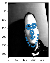
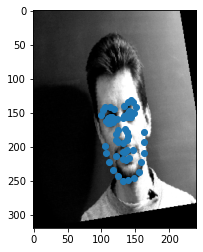
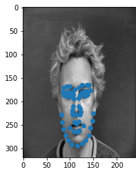
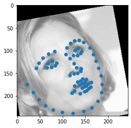
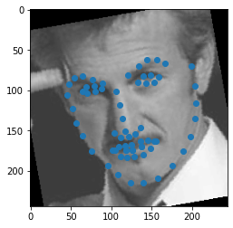
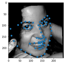
With these augmentations, we now have images as follows:
Improving Model Architecture
There are a series of modifications that help improve the model architecture to perform better than previously seen.
- Significantly increased the number of channels in the image
- Appended a sigmoid layer at the end to set the final values between 0 and 1
- Added a dropout layer to our Fully Connected network to combat overfitting
First, by increasing the number of channels, our network becomes more expressable and is able to capture a greater number of features useful for later layers. Our
architecture now looks as follows:
- A 5 X 5 convolutional layer from 1 channel to 20 channels
- A 5 X 5 convolutional layer from 20 channels to 40 channels
- A 5 X 5 convolutional layer from 40 channels to 80 channels
- A 3 X 3 convolutional layer from 80 channels to 160 channels
- A 3 X 3 convolutional layer from 160 channels to 320 channels
- A 3 X 3 convolutional layer from 320 channels to 320 channels
- A fully connected layer from 4800 channels to 10000 channels with dropout
- A fully connected layer from 10000 channels to 116 channels
Note: the last convolutional layer does not have a max-pool at the end of it. Otherwise, all convolutional layers contain a ReLU and a max pool. The first fully connected layer has dropout with probabiliy 0.4 with ReLU activation.
The final layer has a sigmoid activation. Our learning rate was tuned to be 0.0001.
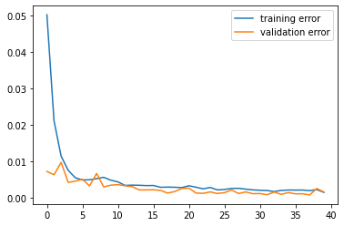
Results
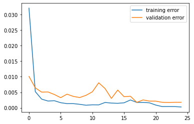
Below is our loss curves:
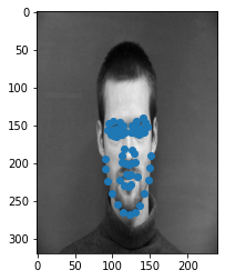
Success Cases
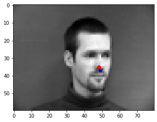
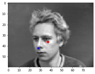
Failure Cases
These failure cases are likely due (once again) to lack of data and improper hyperparameter tuning. In the next section we will use transfer learning to boost our accuracy on a larger
dataset!
Visualization
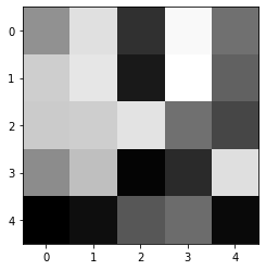
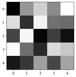
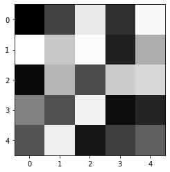
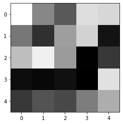
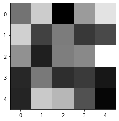
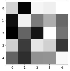
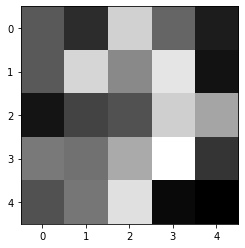
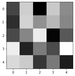
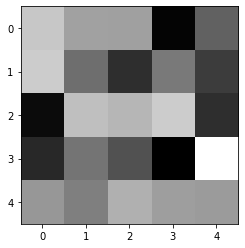
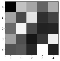
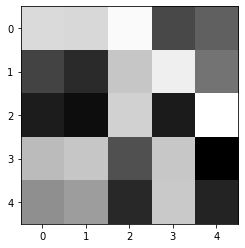
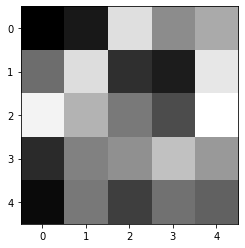
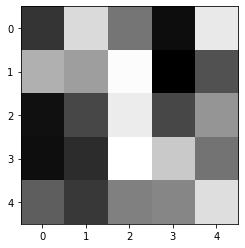
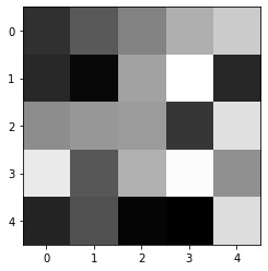
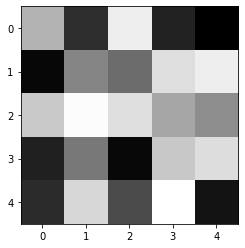
It is interesting to visualize what the learned filters of this model are. We have 20 of them in the first layer, which have shown below.
Of these, the third and eighth filters are interesting since they resemble edge detection filters in the north and south. In general, there is a lot of
heterogeneity in these filters but it is noticable that between any two squares there is usually a lot of contrast. This suggests a high reliance on edge detection
to help with keypoint detection!
Trasfer Learning to Boost Keypoint Detection
To boost our keypoint detection to superhuman levels, we will use the method of simplicity: cheating. In other words we will take an already pretrained neural network on a
larger dataset and use the learned features to train a new neural network that will better fit the edge case, which is keypoint detection.
Dataloader
For this, the only major challenge was utilizing bounding box data along with the image data to crop our images so that they had the face inside of them.
There were certainly cases in which the keypoints actually existed outside the bounding box. For this reason, we resized our bounding box to be 40% bigger in the x and y directions. Here are some images from our dataset.
Model Architecture
We utilize the ResNet-18 model making two very simple modifications:
-
The first layer is a convolutional layer that takes in 1 channel instead of three
-
The final layer is a fully connected layer that outputs 136 points, one for each coordinate of the keypoint.
Other than that, the architecture is the same as ResNet which includes a lot of Batch-Normalization layers and Residual layers with skip connections.
Since this model is bigger, it also requries us to train it for a lot longer! With our augmented data-set however we don't neet to train for too long before our
network starts performing well.
We trained the model for 10 epochs with a learning rate of 0.0001 and then reduced the learning rate to 0.00001 and trained it for another 3 epochs. This works out well
since the reduction of the learning rate helps the network fine-tune its predictions without overfitting too much.
Results
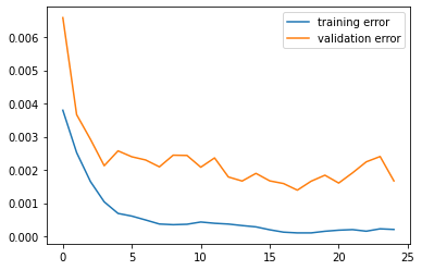
Below is our loss curve. Note that the losses are much much lower now!:
Here are some of our faces that we were able to predict from the test set!
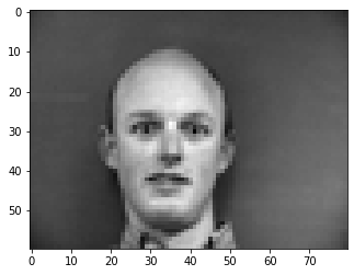
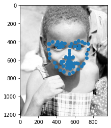
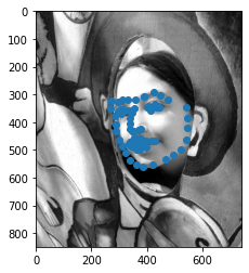
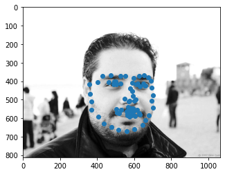
Here are some of my personal images that were predicable here. The first is me, the second is me when I was 5 years old, and the third is my dad!
We note that this model does really well on the one in the middle and a bit more sub par on the two outside. I think the last one is particularly poor simply because the image quality
is low. That image in particular was upsampled to 224 by 224 where as the other two were slightly downsampled. Overall, however, the network does fairly well in identifying keypoints.
Finally, we reported our resuts on Kaggle and received a score of:
10.16687 among the top 40 students!