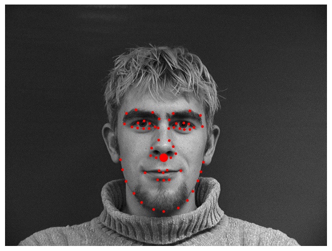
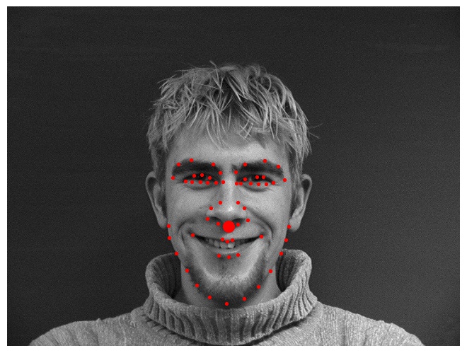
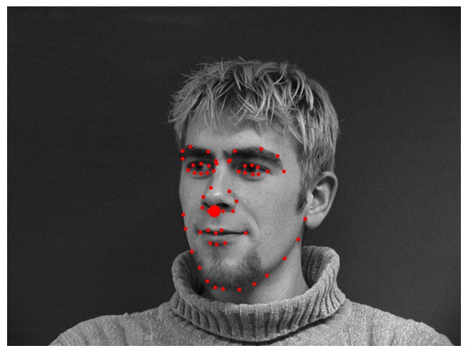
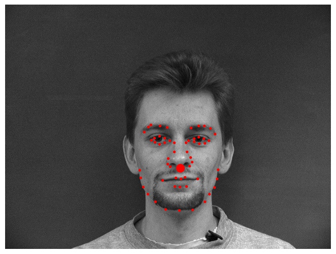
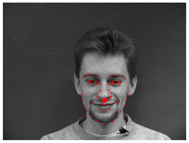
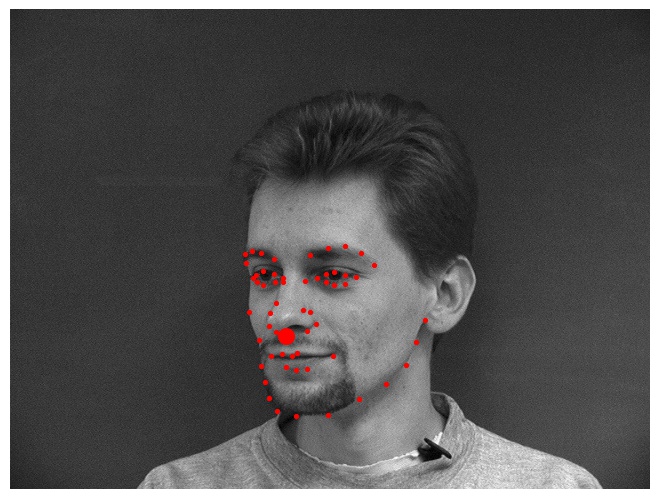
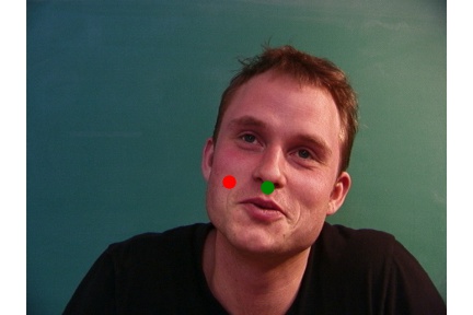
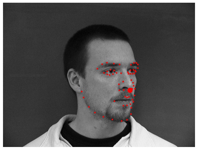
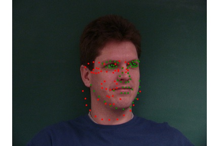
We will first sample some images from my dataloader and visualize it with
ground-truth keypoints given by the dataset. We will plot both the landmark
points and the nose keypoint.
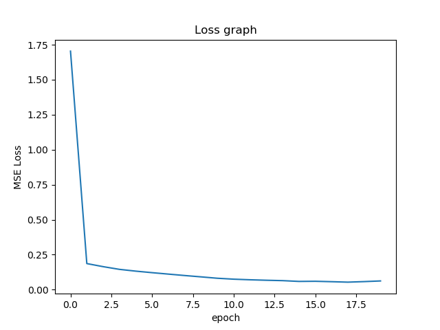
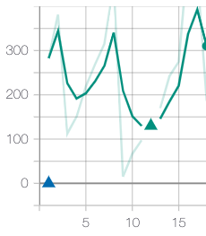
Now, we will plot the train and validation accuracy during the training
process for both the training dataset and the validation data set. The
neural network that I made is similar to a LeNet-5. It has 3 Convulation
Layers followed by 2 Fully connected layers. During the training process, we
use a Adam Optimizer, with learning rate 0.001 and run for 20 epochs.
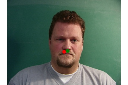
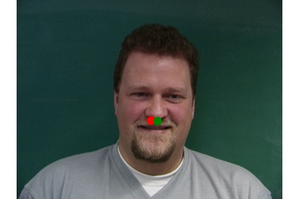
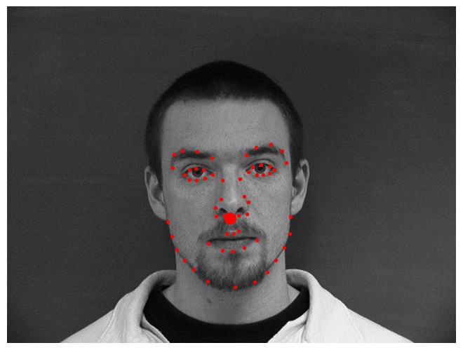
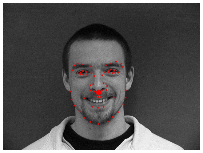
Finally, I will show how 3 facial images which the network detects the nose
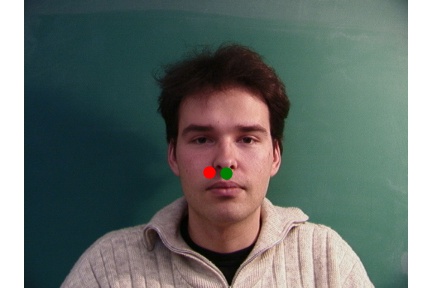
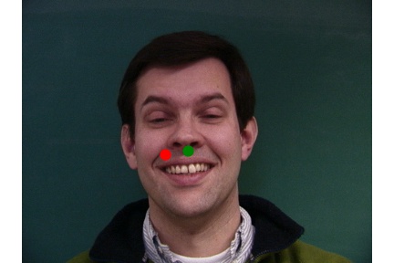
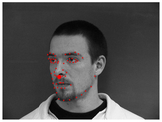
correctly, or fairly reasonably close, and 2 more images where it detects
incorrectly - way off. I believe there some images are predicted well becase
some the training data does not have enough data and doesnt generalize well
for various images with different angles or with various positions of where
the face is positioned in the image.
Fairly Good results
Fairly Bad results
Part 2
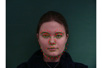
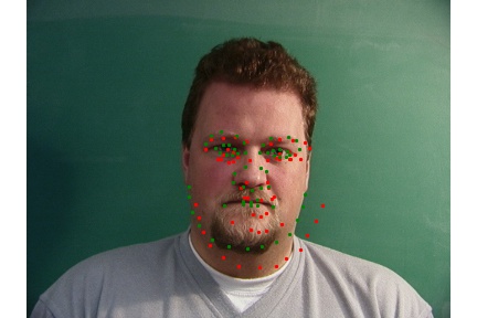
Sampling some truth images from the dataloader
Again, we will first sample some images from my dataloader and visualize it
with ground-truth keypoints given by the dataset. We will plot both the
landmark points and the nose keypoint.
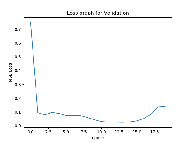
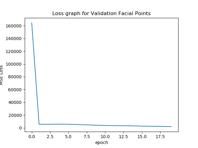
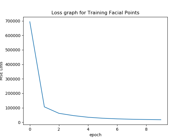
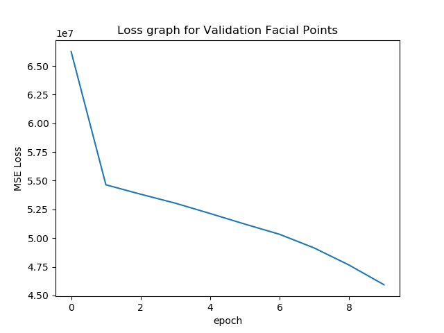
Accuracy i.e Loss Graphs in this project
Now, we will plot the train and validation accuracy during the training
process for both the training dataset and the validation data set. We can
see that they both go down drasticaly and plateuu around some convex point.
According to the validationg raph, we might have picked a learning rate that
is too high.
Architecture
The neural network that I made is similar to a LeNet-5. It has 5 Convulation
Layers followed by 2 Fully connected layers. During the training process, we
use a Adam Optimizer, with learning rate 0.001 and run for 20 epochs. The
architecture of my neural network is based on the Resnet18. I simply changed
the conv layer 1 and the FC layer to take in images that are grayscale and
to output a tensor of shape 136,. The hyperparameters is the interesting
part. I tried a lot of various hyperparameters, i.e diff learning rates
(between 0.001 and 0.0001) and different batch sizes (6, 8, 256), and
different epochs (10, 20, 25). I was very limited by compute because it took
around 4-5 hours to train 20 epochs at various hyperparameters. I also tried
various transforms, but it turned out that the least amount of transforms,
i.e Gray, and Normalization, worked best on the test set. I also tried
rotation and coloring randomization but it seemed to not improve
performance.
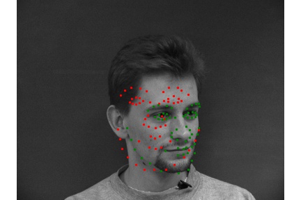
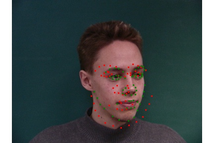
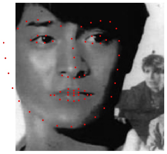
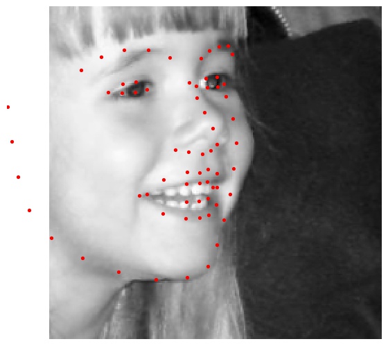
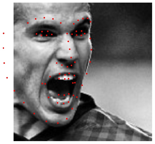
Now, we will display some images predicted by the CNN that I mentioned
earlier. The top 2 images show facial images which the network detects the
nose correctly, and the bottom 2 images show more images where it detects
incorrectly. I believe there some images are predicted well becase some the
training data does not have enough data and doesnt generalize well for
various images with different angles or with various positions of where the
face is positioned in the image. Especially since the output vector is of
larger space, i.e a vector of 58 number for each single sample, we need more
data to train the network. Thus, there are still a lot of inaccuracies.
Fairly Good results
Fairly Bad results
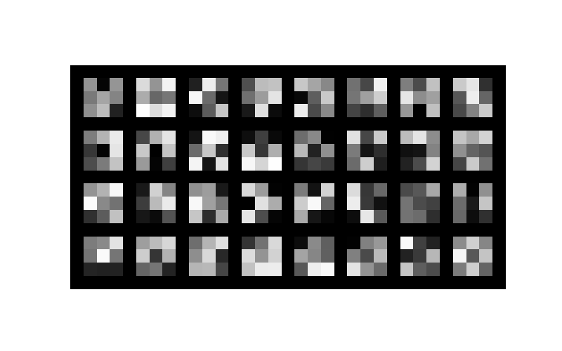
Finally, we will visualize the Convolutional Layer filters, from Layer 1,
Layer 2, and Layer 3. Here are the filters that are visualized in a grid
structure with some of the convolutional layer filters visualized.
Part 3 Train with Larger Dataset
For the large dataset and the Kaggle submission, I scored a MSE of 8.79, at
3rd place at current time of writing this. It is evident that a smaller
neural network with the right hyperparameters is sufficient to predict
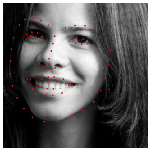
landmarks well. For this part, we will use a larger dataset, specifically
the ibug face in the wild dataset for training a facial keypoints detector.
This dataset contains 6666 images of varying image sizes, and each image has
68 annotated facial keypoints. The neural network used was a Resnet18, with
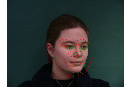
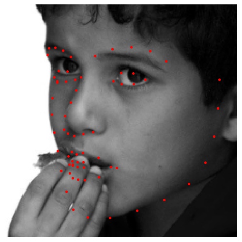
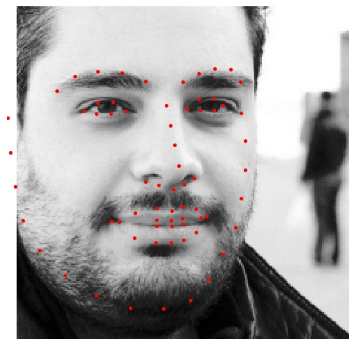
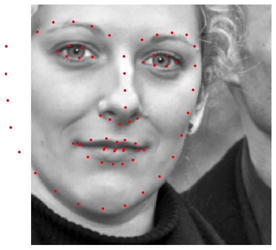
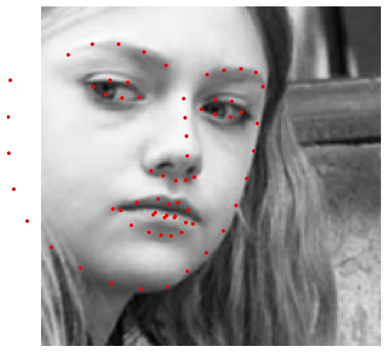
the input layer changed and the output layer changed. Here are images with
the predicted landmarks that were predicted from the test set.
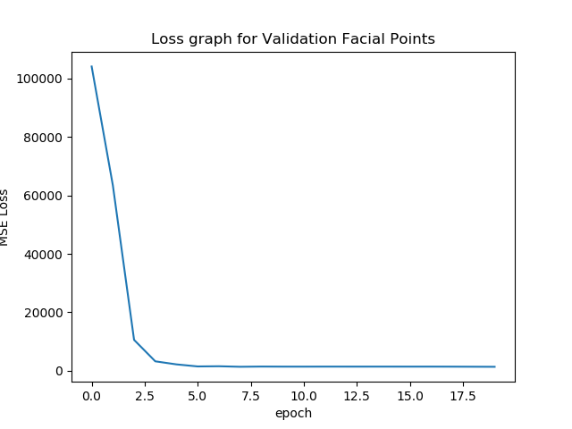
The following is the loss graph that is characterized by the above mentioned
neural network with the above hyperparameters
Architecture
The architecture of my neural network is based on the Resnet18. I simply
changed the conv layer 1 and the FC layer to take in images that are
grayscale and to output a tensor of shape 136,. The hyperparameters is the
interesting part. I tried a lot of various hyperparameters, i.e diff
learning rates (between 0.001 and 0.0001) and different batch sizes (6, 8,
256), and different epochs (10, 20, 25). I was very limited by compute
because it took around 4-5 hours to train 20 epochs at various
hyperparameters. I also tried various transforms, but it turned out that the
least amount of transforms, i.e Gray, and Normalization, worked best on the
test set. I also tried rotation and coloring randomization but it seemed to
not improve performance.
Compute
I used the free tier of Google Colab but made sure to get the Tesla T4. I
hyperoptimized both the GPU and CPU by loading all data into RAM so we can
get O(1) fast access through caching, and I used mixed-precision from
NVIDIA's APEX to reduce the GPU memory necessary so I can load up 128 Batch
size no problem. This led me to compute each epoch in 48 seconds. Thus, 100
epochs ran under 1 hour.
New Architecture - After Making Compute Efficient
Now that I had optimized compute, i.e running 45 seconds per epoch, I got to
try a lot of things. I wrote these down in the Bells and Whistles too. I was
able to also try RESNET50. I loaded the pretrained model from pytorch and
tuned it for 100 epochs. For an odd reason, I couldnt get the output to work
correctly and did not submit to Kaggle with this particular model. However,
it was clear that the valid loss for the Resnet50 at 100 epochs was far
superior to the Resnet50 and 10 epochs. (obviously).
Hyperparameters
Epochs: 100
Learning Rate: 0.05
Batch Size: 128 for both validation and training
Output images on testset.
Bells and Whistles 1 - Anti-aliased max pool.
Modern convolutional networks are not shift-invariant, as small input shifts
or translations can cause drastic changes in the output. Commonly used
downsampling methods, such as max-pooling, strided-convolution, and
average-pooling, ignore the sampling theorem. For this Bells and Whistle, I
used the antialiased-cnns package from
https://richzhang.github.io/antialiased-cnns/.
Dataset
For this part I used the same dataset as from part 3: the ibug dataset of
6666 images.
Neural Architecture
I compared two neural networks and compared them side. The first neural
network I used was a Antialiased-cnns RESNET50 model. I instantiated it like
this.
net = antialiased_cnns.resnet50(pretrained=True, filter_size=4)
net.conv1 = nn.Conv2d(1, 64, kernel_size=7, stride=2, padding=3, bias=False)
net.fc = nn.Linear(2048, 116)
criterion = nn.MSELoss()
optimizer = optim.Adam(net.parameters(), lr=0.001)
net = net.double()
I compared this antialiased neural network with the vanilla counterpart. The
out of the box, RESNET50.
Hyperparameters
Epochs: 100
Learning Rate: 0.05
Batch Size: 128 for both validation and training
Compute
I used the free tier of Google Colab but made sure to get the Tesla T4. I
hyperoptimized both the GPU and CPU by loading all data into RAM so we can
get O(1) fast access through caching, and I used mixed-precision from
NVIDIA's APEX to reduce the GPU memory necessary so I can load up 128 Batch
size no problem. This led me to compute each epoch in 48 seconds. Thus, 100
epochs ran under 1 hour.
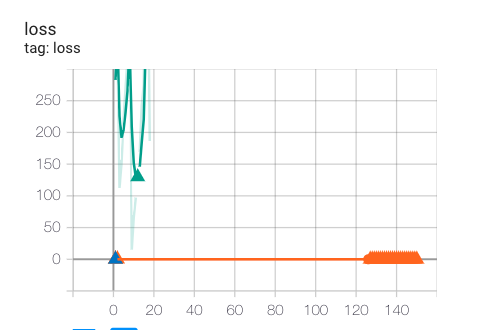
Loss Comparison
The following graphs are graphed with tensorboard in pytorch. Graphing the
validation loss per epoch.
Performance
As you can see from the graph, the performance was around the same - They
both hit the minimum valid loss at around 88. Since I was computing with
mixed precision, the model gradients blew up and became NAN after around 30
or 40 epochs. This is why the graph is not shown for anything after 40
epochs due to the results being NAN due to precision errors. It seems that
with more epochs, the antialias network could perform better, but due to the
APEX limitations of the network, I could not test further with the compute
speed that I desired.
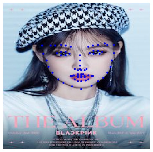
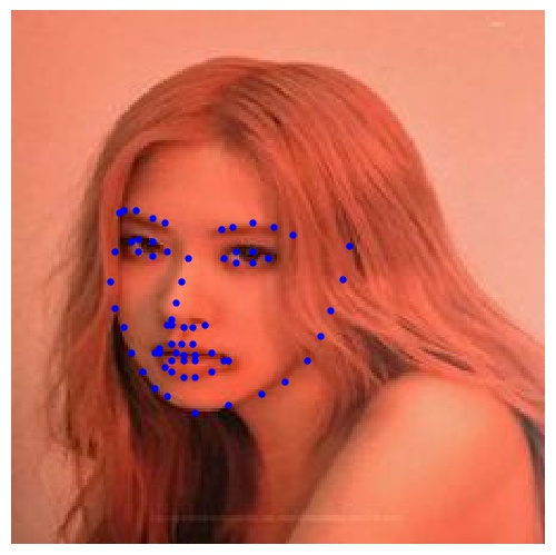
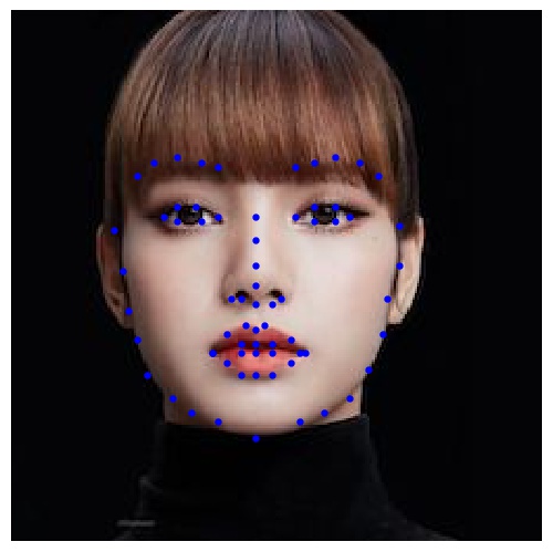
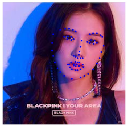
Bells and Whistles 2 - Facial Landmarks + Morphing Sequence
Output images on my favorite ladies.
For this bell and whistle, I took some images of the most beautiful woman
[blackpink] and did facial landmark recognition with the model i had above.
then, I used the morph sequence from the previous project to make a GIF.
Here it is!. We can see that for the images that dont have any face
coverings, the facial points are spot on. However, when there is hair
covering the face, the points can obscure and hard to determine if those
points are in the right location from true points. It is clear that since
most of the images trained had no face coverings, i.e the hair was away from
the face, the network will perform better on images that also have clear
points of face
Another Blackpink Morph
Because blackpink deserves highquality morphs, I took very high resolution
album pictures, and morphed them the same way i described above. The file
size was quite large so I uploaded to IMGUR. Please click this link to see
the second morph
HIGH QUALITY BLACKPINK MORPH