|
|
|
|
Sick of defining points by hand, we've shifted our vision to automatically predicting facial key-points using Convolutional Neural Networks. This was a pretty great experience for me (being the machine learning novice that I am), and I learned a lot about the mechanics of developing machine learning algorithms with PyTorch. I still feel like there is a vast amount of theoretical understanding that I'm lacking, and machine learning is a super rich and mathematically dense field, but hopefully I'll be able to bridge that gap in the future.
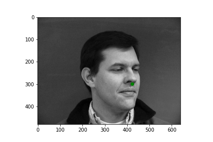
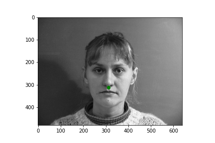
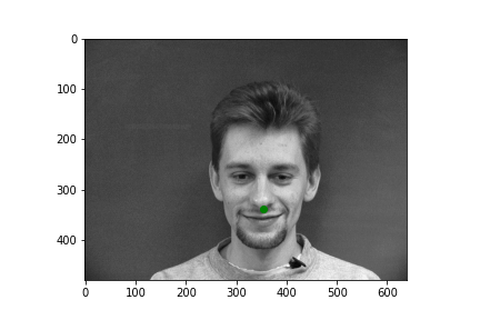
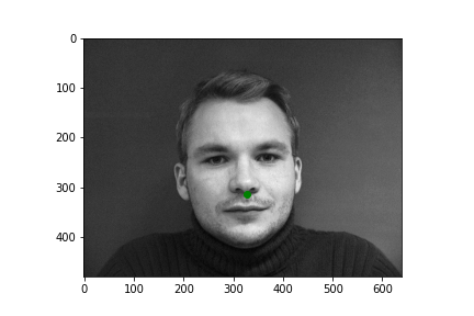
Generating a dataloader is relatively straight forward. We use this dataloader object in order to abstract away a lot of the annoying peculiarities of working with serial data. Namely the dataloader will significantly ease the difficulty of creating batched data, randomizing data ordering, etc. After creating the dataloader in correspondence with the following walkthrough, I can easily sample some input images with their nose point plotted. All images for this part come from the wonderful IMM Face Database. Take a look at some examples.
|
|
|
|
|
|
Next we should actually make our CNN. I've described the underlying structure in the table below.
| Layer | Type | Dimensions (Input, Output) | Kernel Size | Activation |
|---|---|---|---|---|
| 0 | Convolutional | (1, 12) | 3x3 | Relu |
| 1 | Convolutional | (12, 25) | 3x3 | Relu |
| 2 | Max-Pooling | N/A | 2x2 | N/A |
| 3 | Convolutional | (25, 32) | 3x3 | Relu |
| 4 | Convolutional | (32, 32) | 3x3 | Relu |
| 5 | Max-Pooling | N/A | 2x2 | N/A |
| 6 | Linear | (6528, 120) | N/A | Relu |
| 7 | Linear | (120, 2) | N/A | N/A |
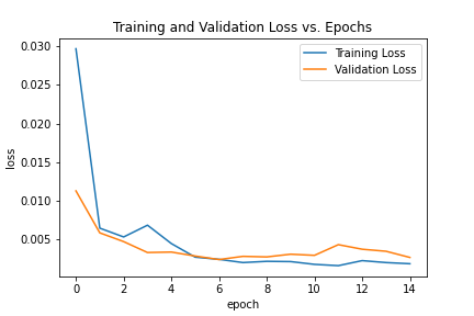
Now let's take a look at how it trained. First, we'll take a look at how the training and validation loss varied on a per-epoch timeline.
|
Not too bad! Although we might see a bit of over-fitting at the end, and it isn't a super representative plot, since our dataset isn't quite large enough.
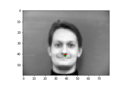
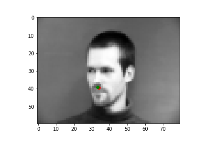
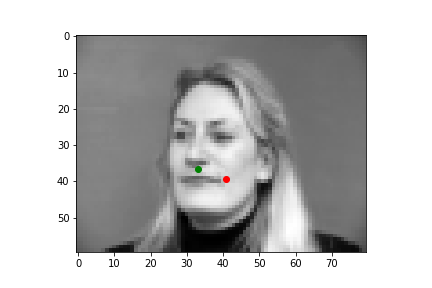
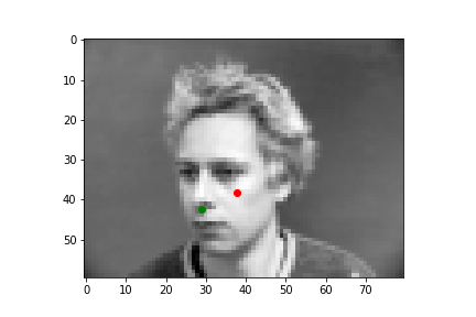
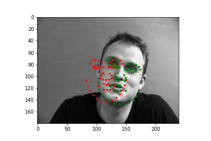
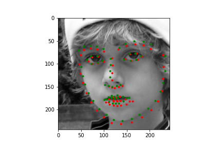
I'll show you four examples below, two where my neural net did a pretty nice job guessing the nose point, and two where it missed the mark. As a note, the green points are the IMM created annotations, and the red points are the predictions the neural net generated.
|
|
|
|
As you can see, the top two predictions are really close! And the bottom two... not so much. Why did it get these wrong? Well the biggest problem is we just don't have enough varied data, which is kind of a cheesy answer because a ton of problems with neural nets are due to a lack of data. But another major issue is you might notice that in the two pictures on the bottom, both individuals are sharply looking to the left, which skews the center point for the face. Especially since we're using a pretty small total dataset, where most pictures are front facing, or pretty close to front facing, our neural net is most likely used to predicting points closer to the center mark, so when the angle of the face is drastically different from the center facing inputs, the neural net has some difficulty.
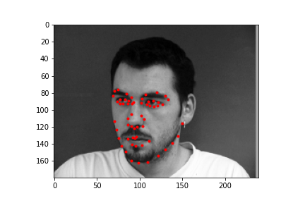
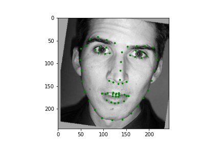
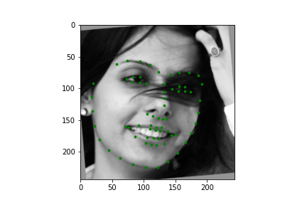
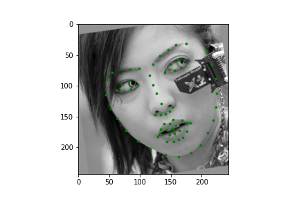
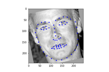
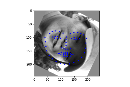
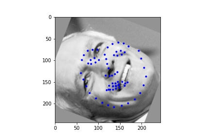
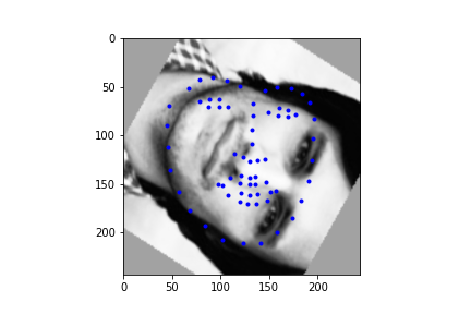
Generating a dataloader the second time around is pretty uneventful so I won't belabor the point too much here. There are only 2 major modifications to be made. The first is for the dataloader to output 58 face points, rather than 1 nose point. Also for data augmentation, our dataloader will randomly rotate an input in the range [-15, 15], and randomly offset the input by 10 pixels in any cardinal direction. Let's take a look at some of the dataloader samples. The points are the IMM selected annotated keypoints.
|
|
|
|
Again, we need to make the actual network, and I'll chart it out in a table below. We're approaching the point of no return with tables; if the networks become vastly more complicated (they will), the tables start to become this cluttered mess, so we'll see how to deal with that later.
| Layer | Type | Dimensions (Input, Output) | Kernel Size | Activation |
|---|---|---|---|---|
| 0 | Convolutional | (1, 12) | 3x3 | Relu |
| 1 | Convolutional | (12, 25) | 3x3 | Relu |
| 2 | Max-Pooling | N/A | 2x2 | N/A |
| 3 | Convolutional | (25, 32) | 3x3 | Relu |
| 4 | Convolutional | (32, 25) | 3x3 | Relu |
| 5 | Max-Pooling | N/A | 2x2 | N/A |
| 6 | Convolutional | (25, 20) | 3x3 | Relu |
| 7 | Convolutional | (20, 15) | 3x3 | Relu |
| 8 | Max-Pooling | N/A | 2x2 | N/A |
| 9 | Linear | (7410, 200) | N/A | Relu |
| 10 | Linear | (200, 116) | N/A | Relu |
| 11 | Linear | (116, 116) | N/A | N/A |
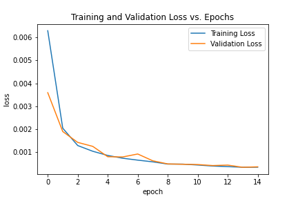
For this neural network, we use the following hyperparameters: epochs = 15, batch_size = 4, learning_rate = 0.0001. We also select
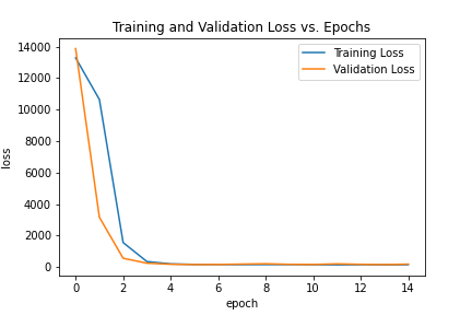
the MSELoss() loss function and the torch.optim.Adam optimizer. As with last time, let's take a look at what happens with the training and validation loss
by epoch.
|
Not much to say, the loss looks fine, but the scale on the left hand side has a wide range, so in actuality, the loss isn't nearly as homogeneous at the end.
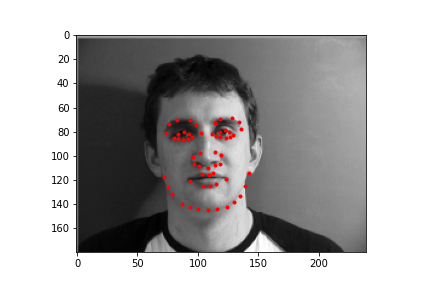
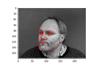
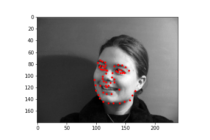
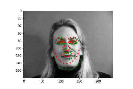
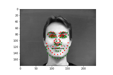
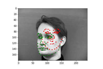
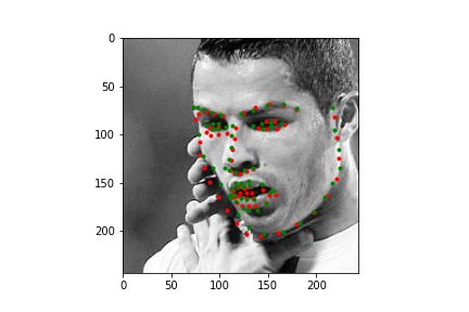
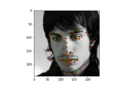
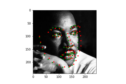
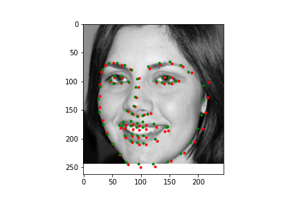
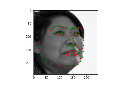
Again, I'll show you four examples below, two where my neural net did a pretty nice job guessing the face points, and two where it missed the mark. Just like before, the green points are the IMM created annotations, and the red points are the predictions the neural net generated.
|
|
|
|
As you can see, the top two predictions are decent. And the bottom two... are relatively bad. Again, probably the biggest problem is we just don't have enough varied data, but also as with last time, a major issue is how these two faces compare to the ones the neural net saw. By and large, most of the faces are relatively centered and angled straight forward, so when the test set has faces that don't follow these majority patterns, it can have a difficult time predicting points, and as you might notice, it tends to predict an average front facing face of keypoints. This is pretty evident in the lower right image, where we have a 3/4 view of the face, and our neural net overlays keypoints over where it thinks the face would be if it were looking straight forward. In the lower left, I wanted to include this output because it highlights a struggling point with networks that don't have enough inputs (even with data augmentation). This definitely wasn't the worst prediction numerically (there are plenty of egregious results to select), but it does represent an issue that is pretty fundamental. Even though there aren't many profile or 3/4 view faces, there are probably less that have these animated poses, like the head lilt in the bottom left. Most likely the fact that this face wasn't straight forward was exacerbated by the fact that there wasn't very much data for predicting these irregular poses.
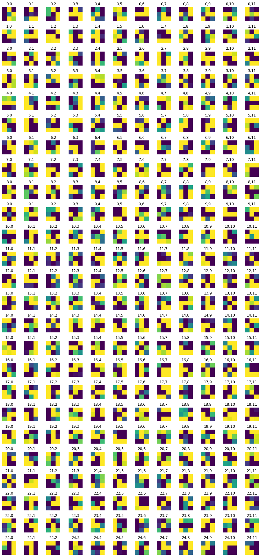
Finally, let's take a look at the learned filters. You can see them for the first and second convolution layers. Pretty interesting! I would have plotted more but as you get deeper into the network, the nature of CNNs is that the number of filters grows drastically, which is too much stress for my poor kernel :(.

|
|
The dataloader from this part is once again derived from the dataloader of the previous section. The only addition is we now crop based on the bounding boxes supplied. To be precise, we crop based on 1.45 times the bounding box. Regardless the process is systematically the same, so there isn't much new here. Let's just look at some samples.
|
|
|
|
We've officially entered the realm of "too complex for tables" so instead I provide the structure dump of the Resnet network.
Below, you can see the architecture of the slightly altered Resnet18 network for the IBug dataset:
ResNet(
  (conv1): Conv2d(1, 64, kernel_size=(7, 7), stride=(2, 2), padding=(3, 3), bias=False)
  (bn1): BatchNorm2d(64, eps=1e-05, momentum=0.1, affine=True, track_running_stats=True)
  (relu): ReLU(inplace=True)
  (maxpool): MaxPool2d(kernel_size=3, stride=2, padding=1, dilation=1, ceil_mode=False)
  (layer1): Sequential(
    (0): BasicBlock(
      (conv1): Conv2d(64, 64, kernel_size=(3, 3), stride=(1, 1), padding=(1, 1), bias=False)
      (bn1): BatchNorm2d(64, eps=1e-05, momentum=0.1, affine=True, track_running_stats=True)
      (relu): ReLU(inplace=True)
      (conv2): Conv2d(64, 64, kernel_size=(3, 3), stride=(1, 1), padding=(1, 1), bias=False)
      (bn2): BatchNorm2d(64, eps=1e-05, momentum=0.1, affine=True, track_running_stats=True)
    )
    (1): BasicBlock(
      (conv1): Conv2d(64, 64, kernel_size=(3, 3), stride=(1, 1), padding=(1, 1), bias=False)
      (bn1): BatchNorm2d(64, eps=1e-05, momentum=0.1, affine=True, track_running_stats=True)
      (relu): ReLU(inplace=True)
      (conv2): Conv2d(64, 64, kernel_size=(3, 3), stride=(1, 1), padding=(1, 1), bias=False)
      (bn2): BatchNorm2d(64, eps=1e-05, momentum=0.1, affine=True, track_running_stats=True)
    )
  )
  (layer2): Sequential(
    (0): BasicBlock(
      (conv1): Conv2d(64, 128, kernel_size=(3, 3), stride=(2, 2), padding=(1, 1), bias=False)
      (bn1): BatchNorm2d(128, eps=1e-05, momentum=0.1, affine=True, track_running_stats=True)
      (relu): ReLU(inplace=True)
      (conv2): Conv2d(128, 128, kernel_size=(3, 3), stride=(1, 1), padding=(1, 1), bias=False)
      (bn2): BatchNorm2d(128, eps=1e-05, momentum=0.1, affine=True, track_running_stats=True)
      (downsample): Sequential(
        (0): Conv2d(64, 128, kernel_size=(1, 1), stride=(2, 2), bias=False)
        (1): BatchNorm2d(128, eps=1e-05, momentum=0.1, affine=True, track_running_stats=True)
      )
    )
    (1): BasicBlock(
      (conv1): Conv2d(128, 128, kernel_size=(3, 3), stride=(1, 1), padding=(1, 1), bias=False)
      (bn1): BatchNorm2d(128, eps=1e-05, momentum=0.1, affine=True, track_running_stats=True)
      (relu): ReLU(inplace=True)
      (conv2): Conv2d(128, 128, kernel_size=(3, 3), stride=(1, 1), padding=(1, 1), bias=False)
      (bn2): BatchNorm2d(128, eps=1e-05, momentum=0.1, affine=True, track_running_stats=True)
    )
  )
  (layer3): Sequential(
    (0): BasicBlock(
      (conv1): Conv2d(128, 256, kernel_size=(3, 3), stride=(2, 2), padding=(1, 1), bias=False)
      (bn1): BatchNorm2d(256, eps=1e-05, momentum=0.1, affine=True, track_running_stats=True)
      (relu): ReLU(inplace=True)
      (conv2): Conv2d(256, 256, kernel_size=(3, 3), stride=(1, 1), padding=(1, 1), bias=False)
      (bn2): BatchNorm2d(256, eps=1e-05, momentum=0.1, affine=True, track_running_stats=True)
      (downsample): Sequential(
        (0): Conv2d(128, 256, kernel_size=(1, 1), stride=(2, 2), bias=False)
        (1): BatchNorm2d(256, eps=1e-05, momentum=0.1, affine=True, track_running_stats=True)
      )
    )
    (1): BasicBlock(
      (conv1): Conv2d(256, 256, kernel_size=(3, 3), stride=(1, 1), padding=(1, 1), bias=False)
      (bn1): BatchNorm2d(256, eps=1e-05, momentum=0.1, affine=True, track_running_stats=True)
      (relu): ReLU(inplace=True)
      (conv2): Conv2d(256, 256, kernel_size=(3, 3), stride=(1, 1), padding=(1, 1), bias=False)
      (bn2): BatchNorm2d(256, eps=1e-05, momentum=0.1, affine=True, track_running_stats=True)
    )
  )
  (layer4): Sequential(
    (0): BasicBlock(
      (conv1): Conv2d(256, 512, kernel_size=(3, 3), stride=(2, 2), padding=(1, 1), bias=False)
      (bn1): BatchNorm2d(512, eps=1e-05, momentum=0.1, affine=True, track_running_stats=True)
      (relu): ReLU(inplace=True)
      (conv2): Conv2d(512, 512, kernel_size=(3, 3), stride=(1, 1), padding=(1, 1), bias=False)
      (bn2): BatchNorm2d(512, eps=1e-05, momentum=0.1, affine=True, track_running_stats=True)
      (downsample): Sequential(
        (0): Conv2d(256, 512, kernel_size=(1, 1), stride=(2, 2), bias=False)
        (1): BatchNorm2d(512, eps=1e-05, momentum=0.1, affine=True, track_running_stats=True)
      )
    )
    (1): BasicBlock(
      (conv1): Conv2d(512, 512, kernel_size=(3, 3), stride=(1, 1), padding=(1, 1), bias=False)
      (bn1): BatchNorm2d(512, eps=1e-05, momentum=0.1, affine=True, track_running_stats=True)
      (relu): ReLU(inplace=True)
      (conv2): Conv2d(512, 512, kernel_size=(3, 3), stride=(1, 1), padding=(1, 1), bias=False)
      (bn2): BatchNorm2d(512, eps=1e-05, momentum=0.1, affine=True, track_running_stats=True)
    )
  )
  (avgpool): AdaptiveAvgPool2d(output_size=(1, 1))
  (fc): Linear(in_features=512, out_features=136, bias=True)
)
For this neural network, we use the following hyperparameters: epochs = 15, batch_size = 4, learning_rate = 0.001. I've also supplemented
this training sequence with a learning rate scheduler, and I've chosen the ReduceLROnPlateau. This has helped me to avoid some drastic overfitting that I was seeing earlier
and for the most part, we can see that the validation and training accuracy lower in tandem, which is great. We also select the MSELoss() loss function and the
torch.optim.Adam optimizer. As with last time, let's take a look at what happens with the training and validation loss by epoch. As I mentioned the training and validation
accuracy are lowering in tandem which is great.
|
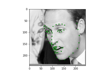
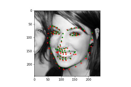
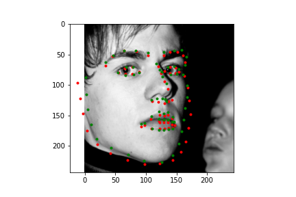
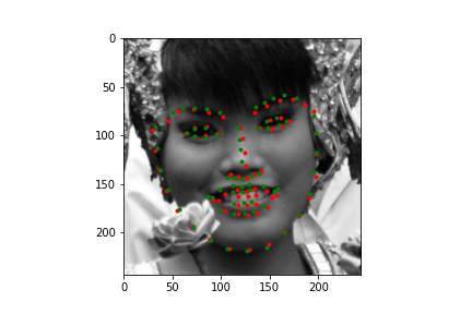
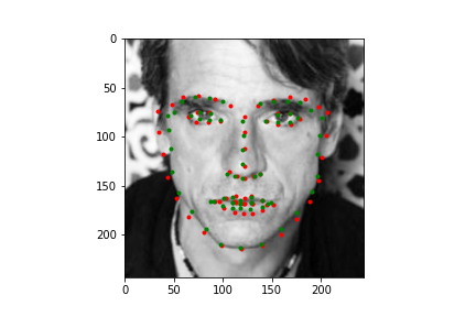
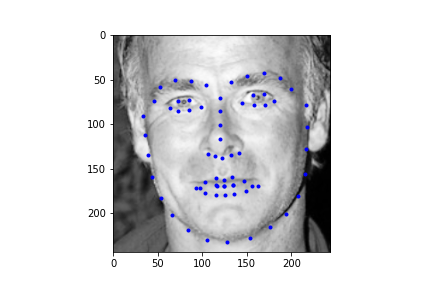
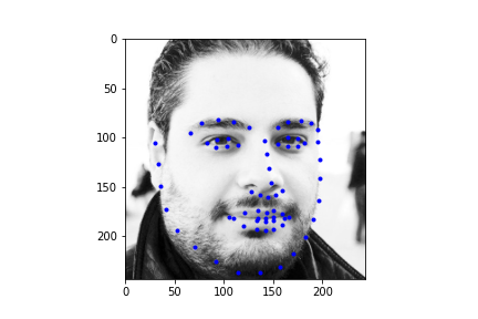
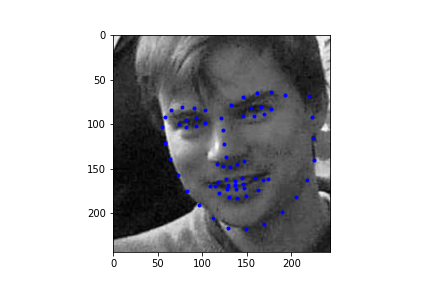
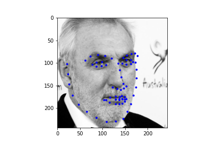
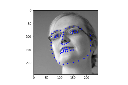
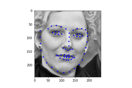
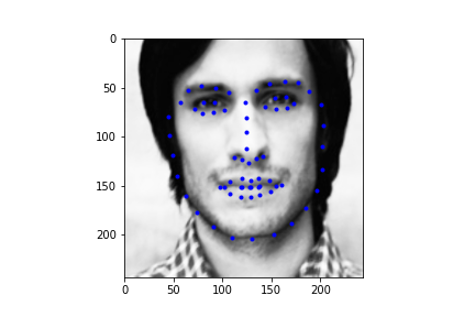
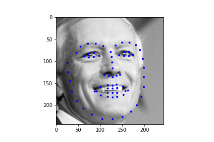
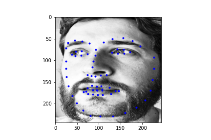
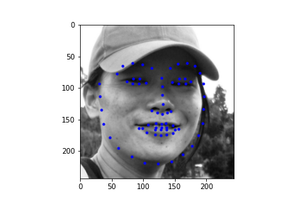
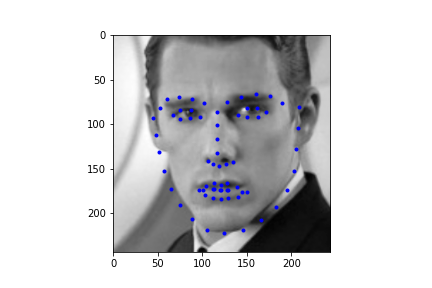
Let's first look at how the neural net predicts some parts of the training set (not best practice I know, but we need annotations, and the test set doesn't have any). Honestly, I'm pretty blown away by this network. It's obviously far from perfect, in large part due to my own inexperience with machine learning, but just how well it can predict face points is a complete marvel to me.
|
|
|
|
|
|
|
|
|
|
Not too bad! The neural net is significantly better at predicting faces, even if the faces are looking to the side, or in profile view, which we can thank in large part to the massive IBug dataset (at least comparatively). It still does a great job getting the straight ahead view as well, and notice that it actually does significantly better at really choosing facial features, rather than seeming like it's trying to average the faces, and predict something that will be close enough. Since there are so many faces at so many angles, with so many different exposures, that sort of logic fails horribly for this dataset which is great. Notice that the net can even predict when people are smiling, or close lipped.
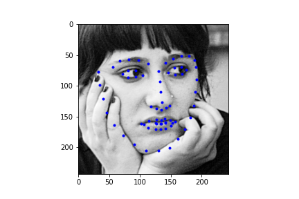
Alright, now finally, let's take a look at some of the regressions our neural net makes for the test set. First I should mention, my Kaggle MAE is around 286. I'm not sure this is truly representative of what my true error is since the face point prediction actually looks half decent, and I have a hunch that I'm making an error with rescaling the points back to the starting image size, but after poking around the CSV generation, I was unable to solve this issue. Regardless, we can take a look at some of the example results below. Also it's totally possible that this IS representative of the actual MAE and my network is just suboptimal (this is actually more likely haha).
|
|
|
|
|
|
|
|
|
|
|
|
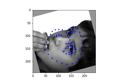
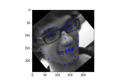
It should be noted though that the efficacy of the net is predicated on reasonable rotations and crops. In other words, break the assumptions of reasonable inputs and you shouldn't expect reasonable outputs. So for instance, here's my neural net's predictions on some testset images again. While images that are mostly vertically aligned tend to work fine, those that have been rotated freely without any real care have some pretty wonky predictions. That's not surprising though. In data augmentation I rotated my images up to 15 degrees clockwise or counter clockwise. Now I'm letting the images rotate freely, so there's bound to be faces that the neural net gets stumped on. The moral of the story is, please give you neural net inputs with at least a semblance of normalcy :') .
|
|
|
|
|
|
All in all, pretty cool, and very exciting for someone who's basically done next to no machine learning in the past :) .