Project 4 - Facial Keypoint Detection with Neural Networks

CS 194-26, UC Berkeley

Yassin Oulad Daoud

Part 1: Nose Tip Detection

For the first part, I wrote a neural network to detect just the nose keypoint.

Dataloader

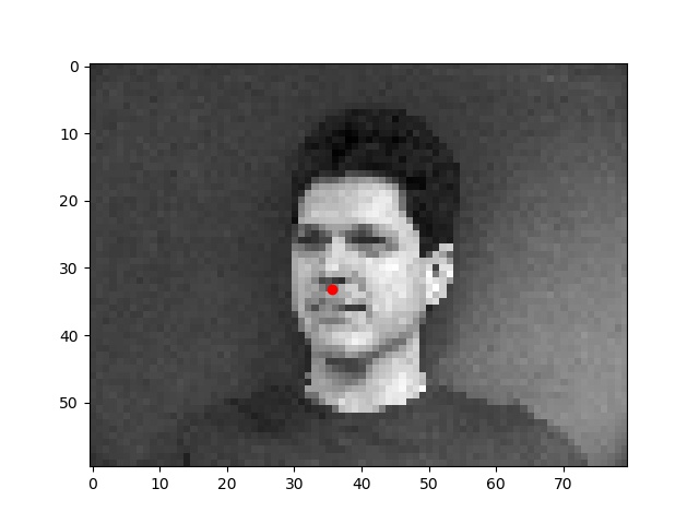
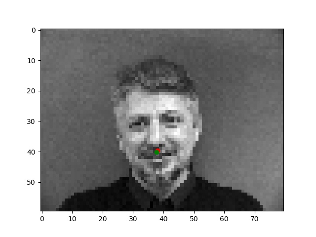
First, I wrote a dataloader to load images from the input dataset, changed their size to 80x60 pixels, and plotted the "groundtruth" nose keypoint in red.

CNN

Then, I defined my neural network, based roughly on the structure of the LeNet network. I had to play around a lot with the structure, and my best run had the following structure:

(conv1): Conv2d(1, 12, kernel_size=(5, 5), stride=(1, 1))
(conv2): Conv2d(12, 16, kernel_size=(5, 5), stride=(1, 1))
(conv3): Conv2d(16, 32, kernel_size=(3, 3), stride=(1, 1))
(conv4): Conv2d(32, 64, kernel_size=(1, 1), stride=(1, 1))
(relu1): ReLU()
(maxp1): MaxPool2d(kernel_size=2, stride=2, padding=0, dilation=1, ceil_mode=False)
(fc1): Linear(in_features=384, out_features=64, bias=True)
(fc2): Linear(in_features=64, out_features=2, bias=True)

Loss function and optimizer

Using nn.MSELoss (mean squared error) as my loss function and the Adam optimizer, I obtained my best results with a learning rate of around 0.00275 - 0.003. A rate of 0.001 fitted the model too slowly and the loss would not drop fast enough, while rates above ~0.003 would produce unreliable results and usually the loss would increase slightly toward the end of the epochs.

Results

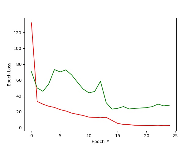
In the loss plot above, the training loss is shown along with the validation loss, each computed as the average MSE between the ground truth point and the network output point for each epoch.

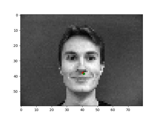
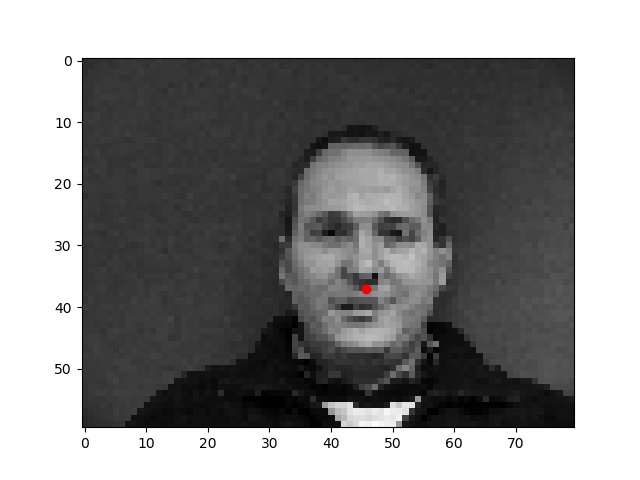
Better results (with the groundtruth nose point and predicted point)

Generally, when the input images had forward-facing poses with straight faces the network yielded the best nose keypoint predictions. There are a higher proportion of these kinds of images in the dataset, so the network was trained to better detect the nose for these kinds of images.

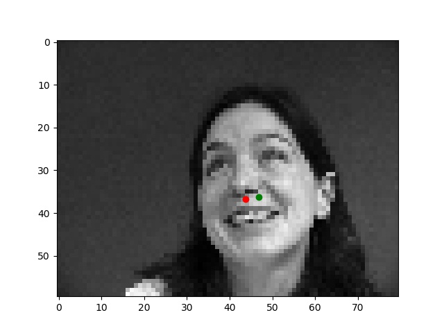
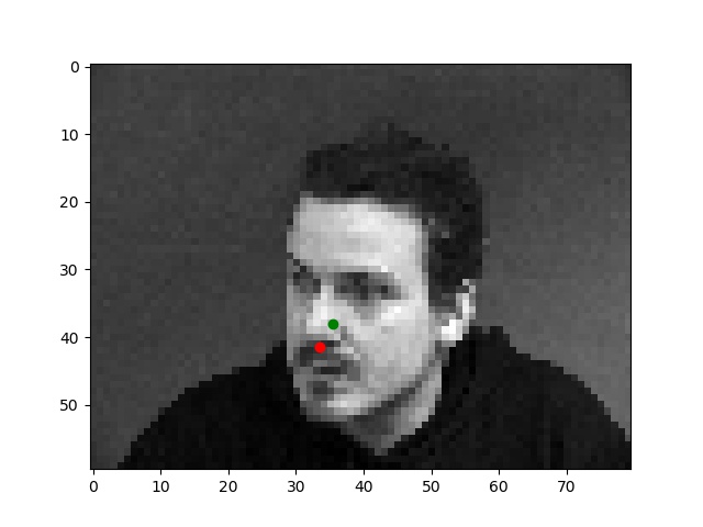
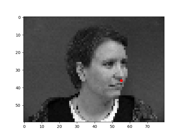
Worse results

When the input images were the "silly"/random pose from the dataset, the network had more trouble finding the nose keypoint. Some of the faces from those input images were rather unique, so the network was more likely to fail on these.

Part 2: Full Facial Keypoint Detection

Dataloader

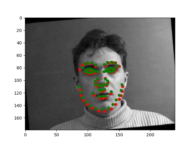
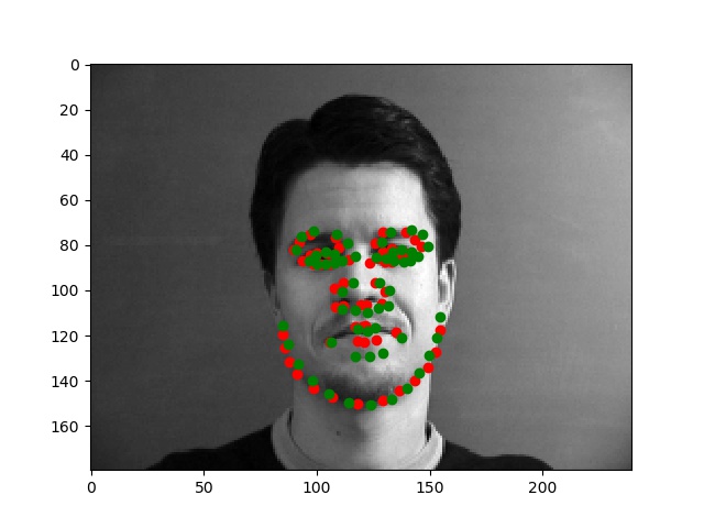
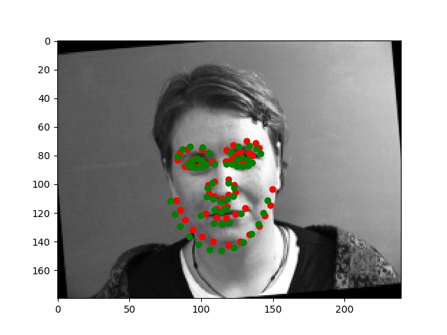
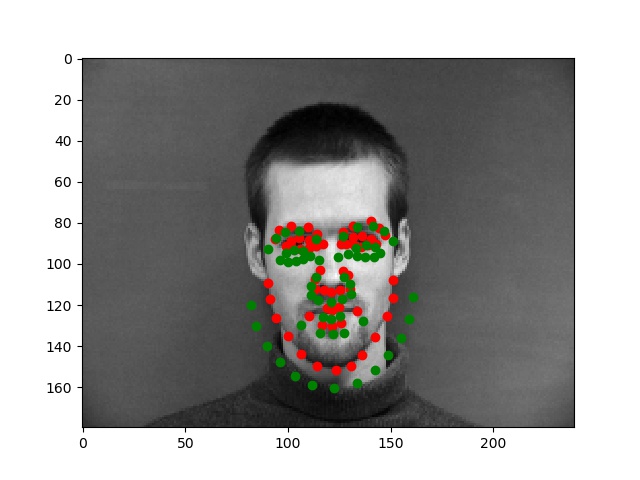
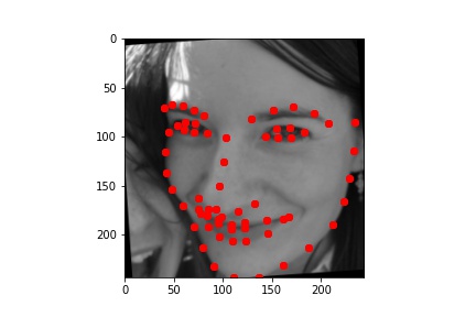
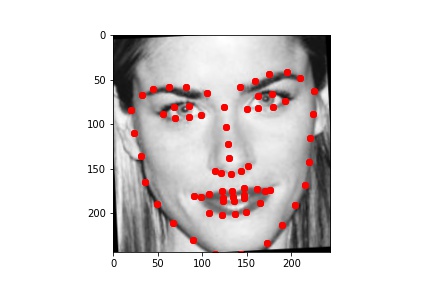
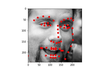
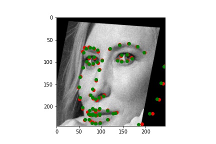
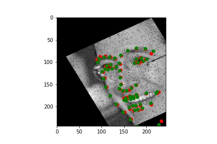
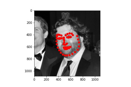
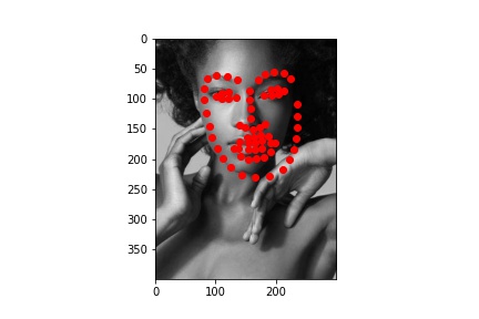
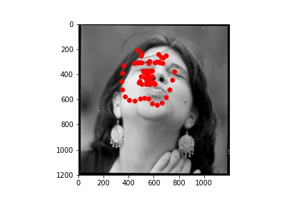
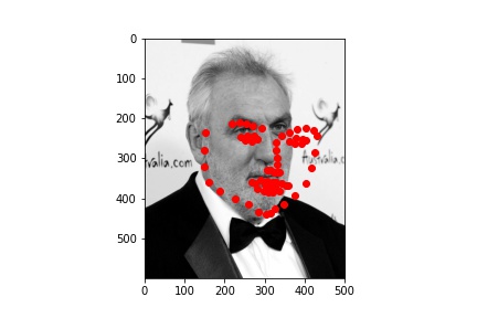
First, I wrote a dataloader to load images from the input dataset and plotted all of the "groundtruth" keypoints in red. This time, I used images of size 160x120, instead of 80x60. I also augmented the dataset, tripling the size of the dataset by including both the original images and 2 randomly transformed images for each of the originals. The transformation was a random slight rotation within [-5, 5] degrees, and a random change in brightness within [50, 150] %. I experimented with cropping, but the keypoints did not adjust to this change well and much of the training data ended up being incorrect as a result, leading to a worse model than without the cropping. Many of the images in the original dataset already have relatively varied face sizes to the cropping transformation was less necessary than rotating and adjusting the pixel values.

Below are a few examples of the images and their adjusted "ground truth" landmarks from the augmented dataset, as used in the training process.

CNN

(conv1): Conv2d(1, 16, kernel_size=(5, 5), stride=(1, 1))
(conv2): Conv2d(16, 32, kernel_size=(3, 3), stride=(1, 1))
(conv3): Conv2d(32, 64, kernel_size=(3, 3), stride=(1, 1))
(conv4): Conv2d(64, 128, kernel_size=(3, 3), stride=(1, 1))
(conv5): Conv2d(128, 256, kernel_size=(3, 3), stride=(1, 1))
(conv6): Conv2d(256, 512, kernel_size=(1, 1), stride=(1, 1))
(relu): ReLU()
(maxp): MaxPool2d(kernel_size=2, stride=2, padding=0, dilation=1, ceil_mode=False)
(fc1): Linear(in_features=1024, out_features=512, bias=True)
(fc2): Linear(in_features=512, out_features=116, bias=True)

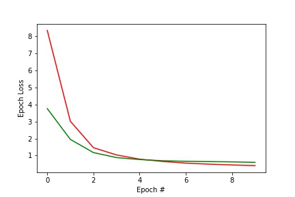
Again, I used the Adam algorithm for my optimizer, this time with a learning rate of 0.001.

Results

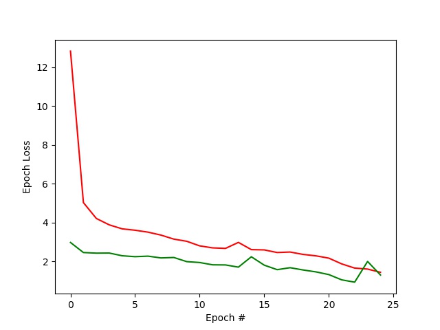
In the loss plot above, the training loss is shown along with the validation loss, each computed as the average MSE between the ground truth point and the network output point for each epoch. I additionally took the average loss per keypoint from each epoch so that the loss metric would be similar to that of part 1, showing the MSE between 1 pair of keypoints rather than the sum over all the 58 keypoints.

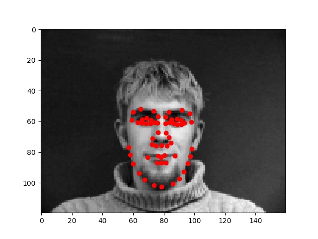
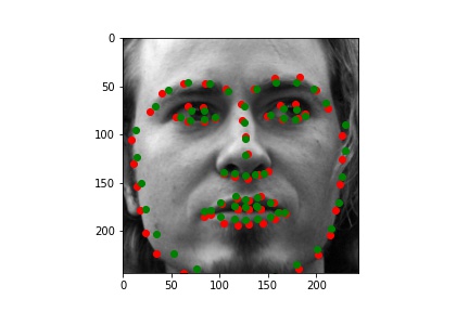
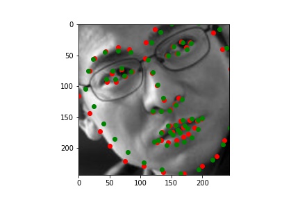
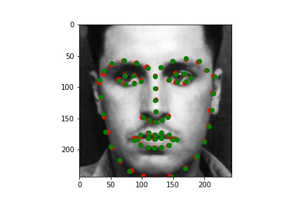
Better results (with the groundtruth keypoints and predicted keypoints)

The results were better for images like these, where the pose is relatively straight and the face is centered. Additionally, these images had darker hair/lighter skin to distinguish the facial features more clearly. In the worse examples below, I noticed an issue with how distinct the face was from the hair/clothing in certain images.

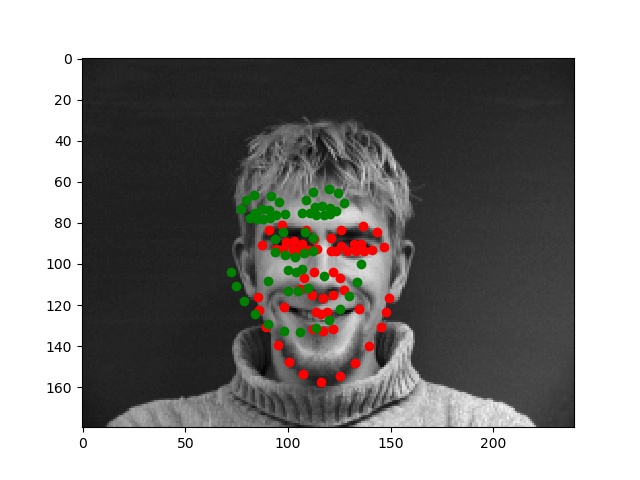
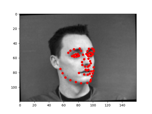
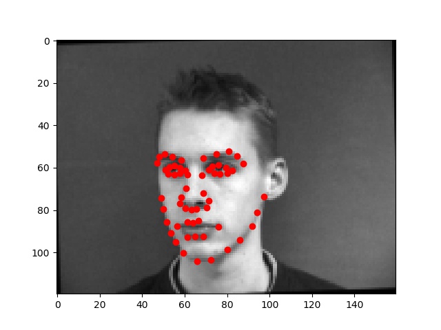
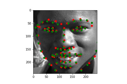
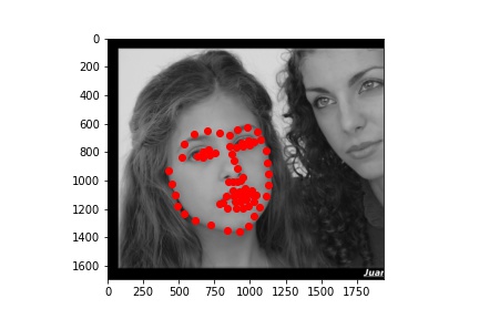
Worse results

These results were worse for various and particular reasons--for instance, for the blonde/highlighted hair of the person on the left above seems to have confused the network, which took parts of the hair and other areas on the face to be facial features. The error on the right, by which the detected keypoints were always somewhat wider and in-line with the shirt collar, kept reoccuring since the person's collar was quite full and distinct (while their facial hair made the real chin look less like a "chin" than the area around the collar). The algorithm kept mistaking the collar for the chin and jaw, while the images that did not have visible/perfectly round shirt collars did not generally have this issue.

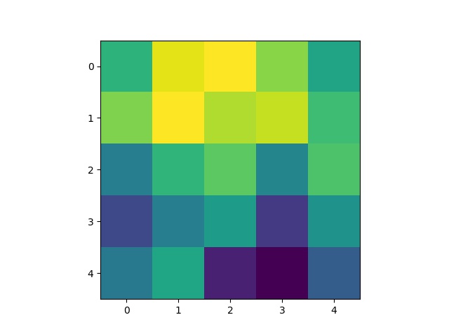
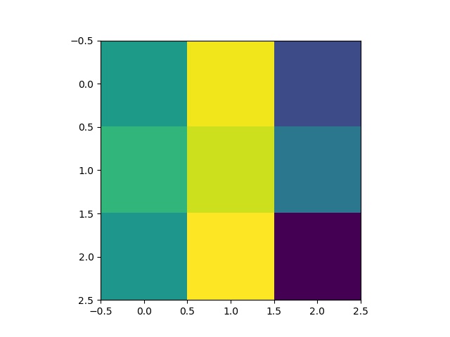
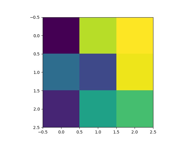
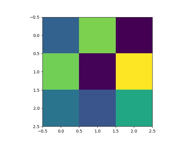
Some 5x5 filters from the 1st layer of the neural network:

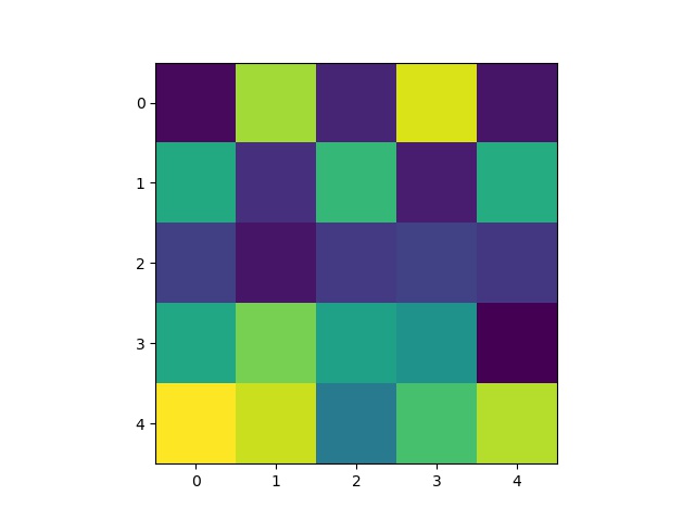
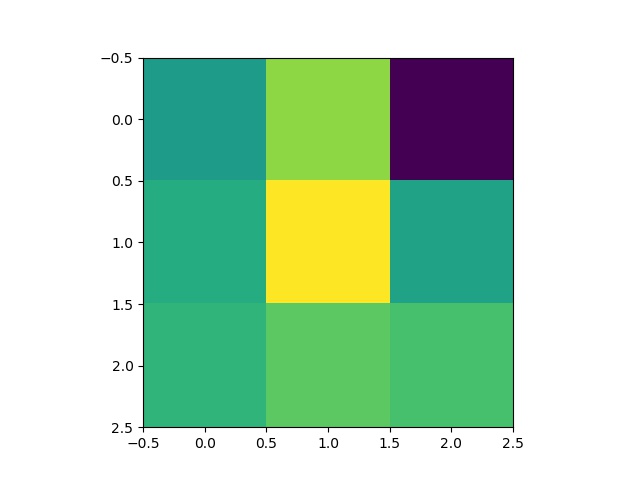
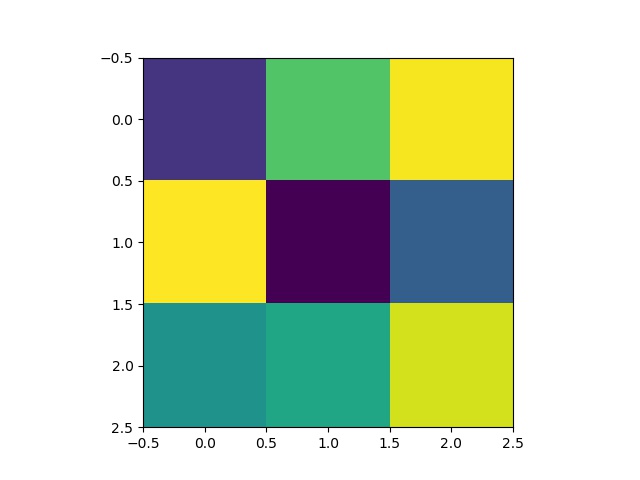
Some 3x3 filters from the 3rd layer of the neural network:

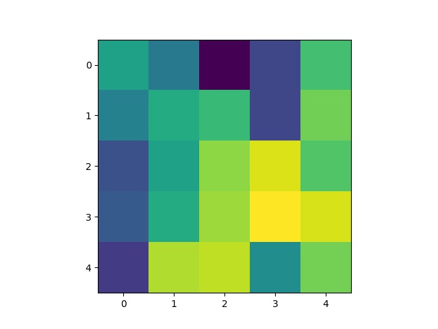
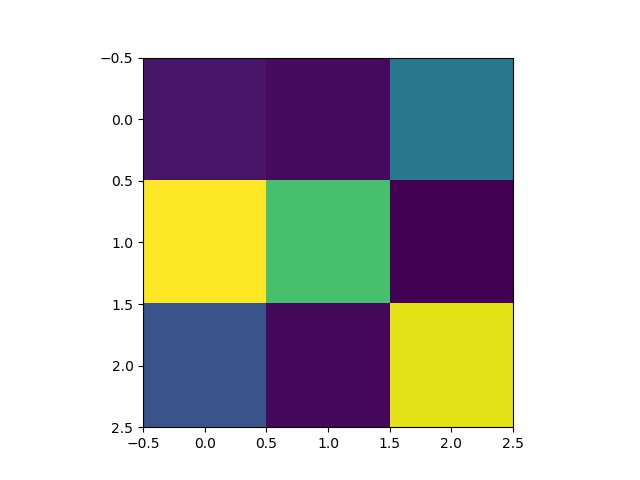
Some 3x3 filters from the 5th layer of the neural network:

Part 3: Training with a Larger Dataset

Dataloader

First, I wrote a dataloader to load images from the input dataset and plotted all of the "groundtruth" keypoints in red. For this part, the image size for the training dataset I used was 244x244. Since the raw input dataset for this part had 6666 images and faces of different sizes, I had to use bounding box coordinates provided by the staff to crop the images just around the face. I then resized the cropped images to 244x244 pixels, and adjusted their landmarks accordingly (by shifting them using the bounding box coordinates and scaling them to the resized image).

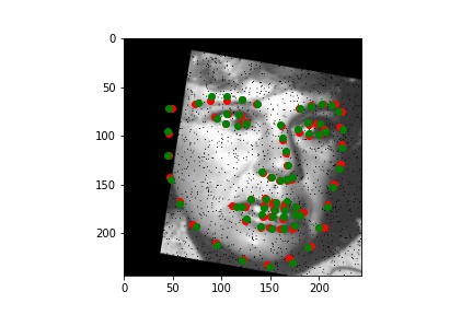
As in part 2, I augmented the dataset, doubling the size by including both the original images and a randomly transformed image for each of the originals. I used the same random transformation to produce the augmented dataset: a random slight rotation within [-5, 5] degrees, and a random change in brightness within [50, 150] %.

Below are a few examples of the images and their adjusted "ground truth" landmarks from the augmented dataset, as used in the training process.

CNN

For this part, I used the pretrained ResNet18 model rather than defining my own CNN. I found that the ResNet18 model was doing quite well at reducing the training and validation loss, and I did not have to change much. Rather, the biggest challege was getting enough data augmentation (and performing the right transformations -- for example, randoms horizontal/vertical flips caused adverse, "averaging" predictions rather than "informed" ones) and running the augmentation repeatedly throughout the training process, while running the ResNet18 training for many epochs. If this rigorous augmentation is not applied, the model would learn to identify just the training images extremely well, and produce near-random results when faced with the test data.

With that, the main changes I made to the model hyperparameters were changing the input # of channels to 1 (because the training images are greyscale, not 3-channel RGB images) and changing the # of output channels to 136 (=68*2 for each of the 68 keypoint x- and y-values). At first, I ran the training loop after setting the kernel size in the first convolutional layer (conv1) to 5x5, but I obtained better results by changing this to 7x7, probably because the wider kernel at the beginning would prevent the model from "overpredicting" during the first layer when faced with noisy/undersirable pixel data I added during augmentation. I used the Adam optimizer as in the previous parts, with a learning rate of 0.001. The model's details are below:

Results

First try

I plotted the training loss and the validation loss, each computed as the average MSE between the ground truth point and the network output point for each epoch. I computed this loss the same way as in part 2, so that it would be easier to see the improvement between using my own CNN on the small dataset to using ResNet18 on a large dataset.

Training set output (with the groundtruth keypoints and predicted keypoints)

I initially ran the ResNet18 training loop for just 10 epochs using a lightly augmented dataset with just a rotation within [-15, 15] degrees and brightness changes I used on the Danes dataset in Part 2. I already achieved pretty good results over the training and validation datasets, but when evaluating the model over the test images, the predictions were pretty poor. This was probably because the test dataset had a variety of images that exceeded the variety rather weak augmentation I performed over the dataset.

Second try: More epochs, more dataset augmentations

This time, I ran the training loop for about 100 more epochs, and every 10 epochs, I re-augmented the dataset using a copy dataset of the original training set from before.

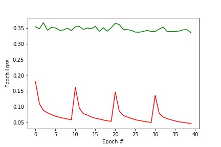
NOTE: I trained for 100 epochs, but unfortunately, after the 60th or so, my runtime crashed for using too much memory, and so I lost the validation/training loss data I had recorded. I reran the training loop for the last 40 epochs, and plotted the training loss and the validation loss above. Becuase I re-augmented the training set every 10 epochs, the loss would jump back up; but with every cycle of 10 epochs my initial prediction got better, so the peaks would drop slowly over time.

For augmentation, I also increased the amount of tranformation I was doing, from just a slight rotation and brightness change in Part 2 to:

Below are the results of the predicitons over the training set, including some examples of the transformations I described.

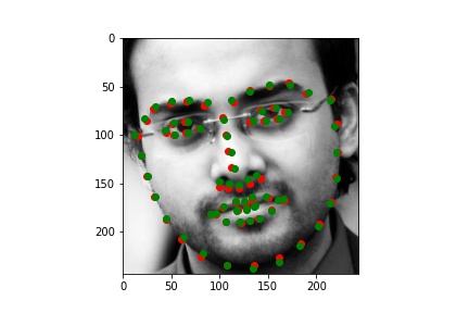
Training output (with the groundtruth keypoints and predicted keypoints)

After training the model, I evaluated the model on the test dataset. Some of the resulting predictions are below:

Better results

Worse results - I found it funny that the person on the left looks as if they are being hit by the incorrect predictions! :D

Self-chosen test images: Early Modern to Modern portraits

As always, working so much with real human faces for these projects, I wanted to have a change and apply my results to paintings! The new test I chose are below:

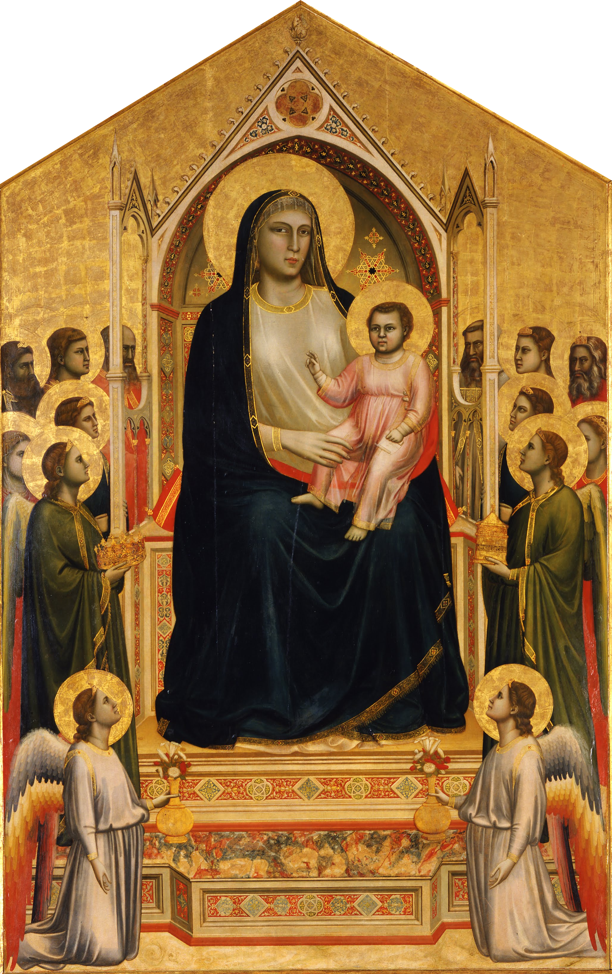
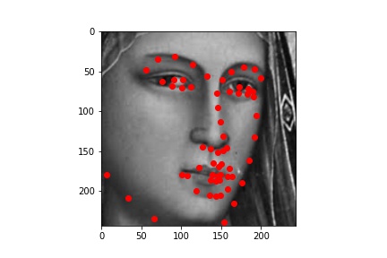
Giotto, Ognissanti Madonna, 1310.

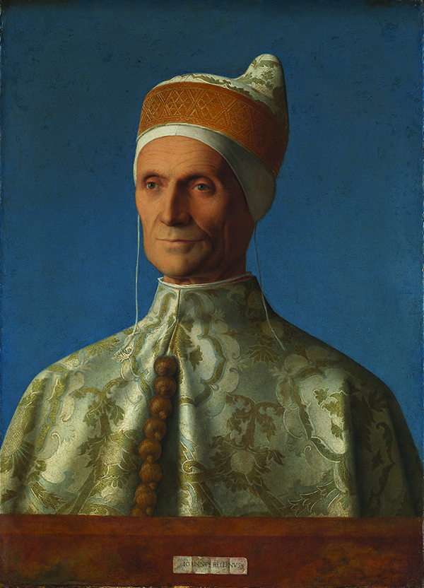
Giovanni Bellini, Portrait of Doge Leonardo Loredan, 1501-2.

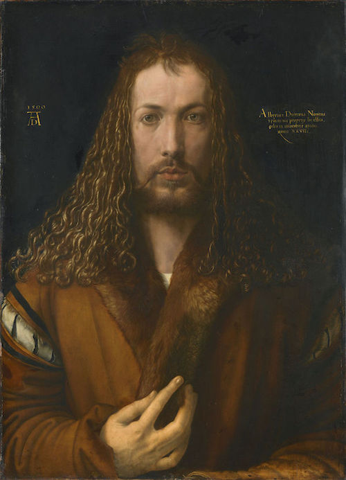
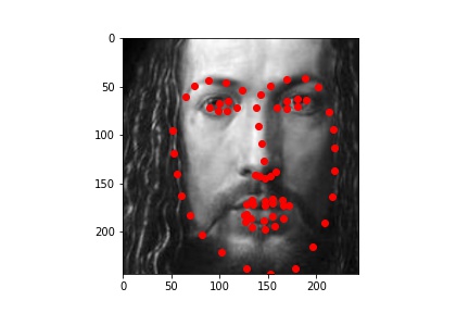
Dürer, Self portrait, 1500.

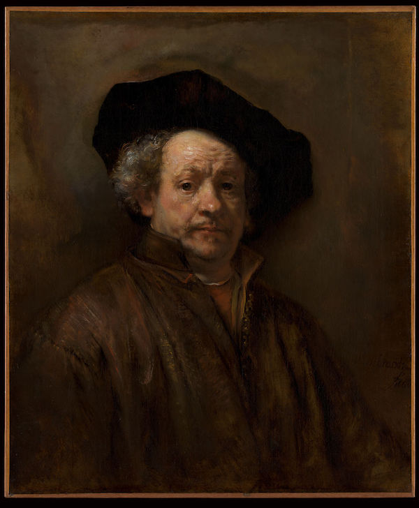
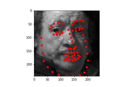
Rembrandt, Self portrait, 1660.

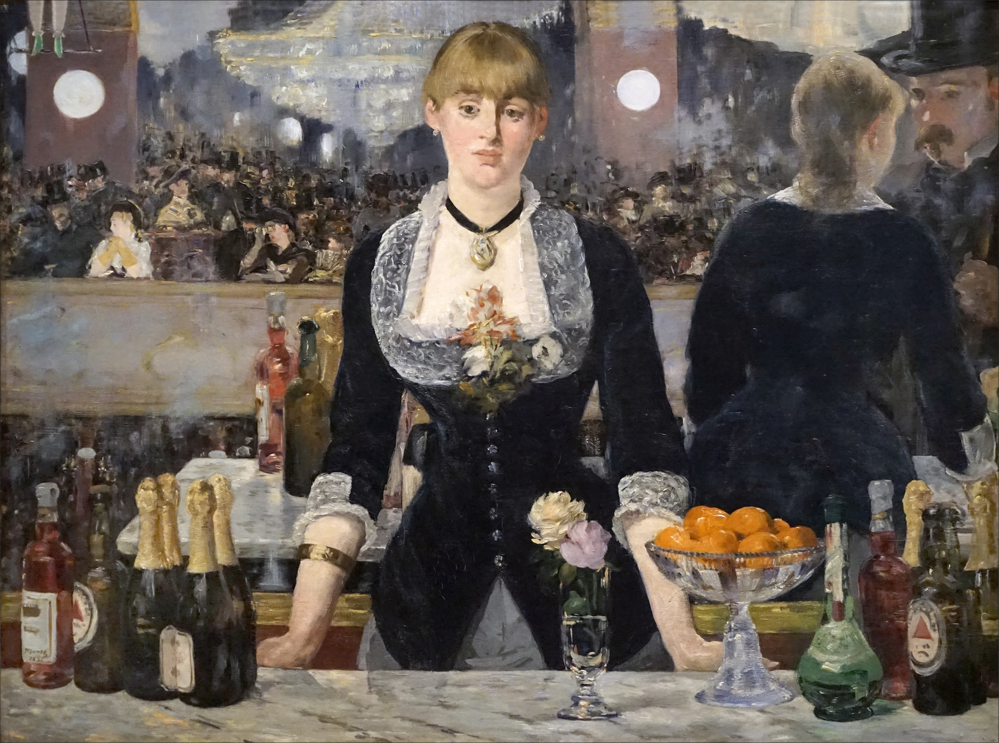
Manet, Bar at the Folies-Bergère, 1882.

I ran the predictions using the trained model, and plotted the predicitons on the images below:

Full-sized output:

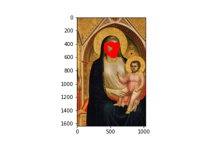
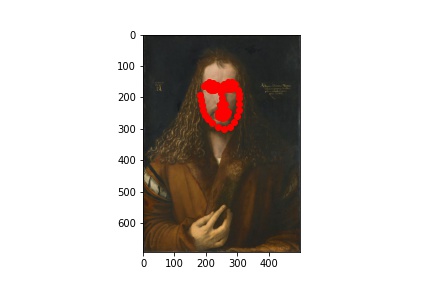
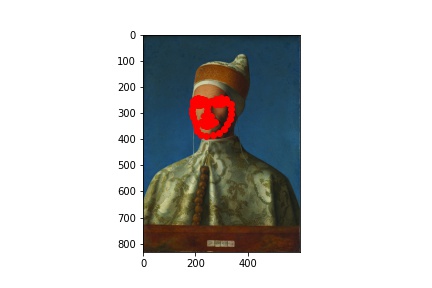
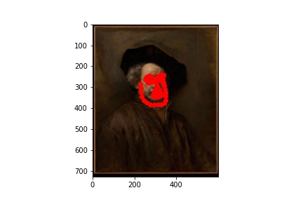
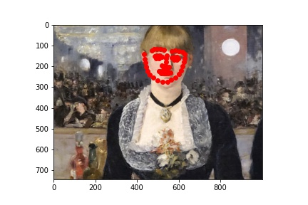
Initially, I had expected the later images (the Rembrandt and the Manet) to not work as well, and it is precisely why I chose them as examples. There is a phenomenon in the tradition of early modern to modern European painting, by which we see (generally) painters go from relying heavily on line/preliminary drawing to depict forms to later (around the Baroque period) relying instead on light value and brushstroke to do the same (culminating in the impressionists and beyond, on whose paintings I did not dare try my model!). The computational recogintion model, relying on gradients of pixel values, would naturally respond better to the line-based compositions. This is why, even though a modern human viewer might point to Rembrandt as painting with greater "naturalism" than did Giotto (and especcialy Giotto's predecessors), the computational predicatbility of paintings doesn't necessarily imply their naturalism.