Project 5 : (Auto)sticthing and photo mosaics

In this project, we will be combining everything that we learned in this semester through working on Mosaics. Specifically, the first part will be about implementing manual stitching. The second part will be about creating an algorithm that performs stitching automatically.

Part A: Image Warping and Mosaicing

This project can basically be divided into four main parts:

1. Data Collection
2. Homography Recovering
3. Inverse Warping and Rectifications
4. Panorama: Blending mosaic

1 - Data Collection

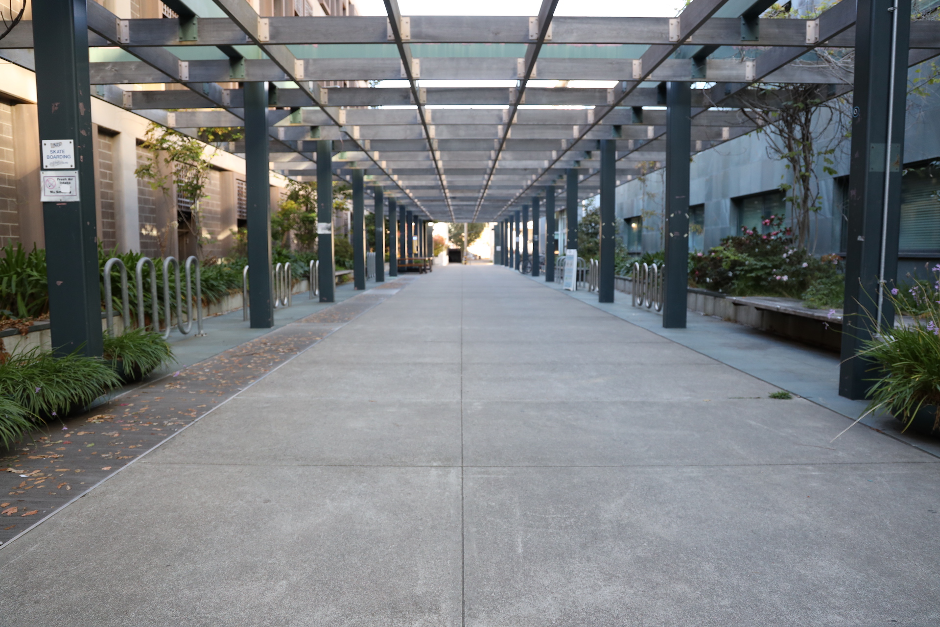
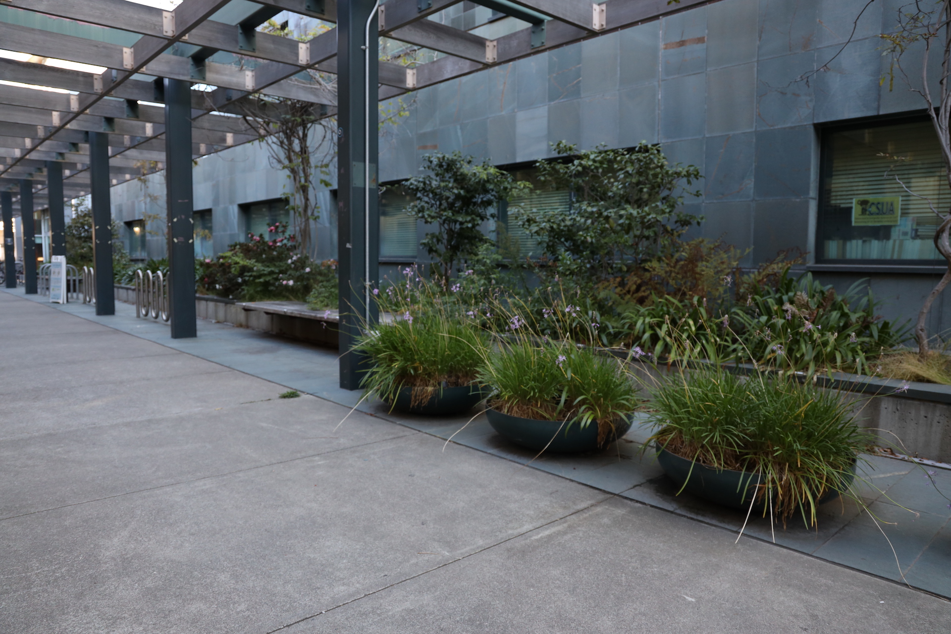
For the purpose of this project, I took out my mirrorless camera and started thinking about where to take picture. I wanted a place that had a lot of features that I could create correspondences on. Additionaly, I wanted to pick a place that has a lot of significance to me. Therefore, I decided to take a series of pictures on a triped with my mirrorless camera in front of Soda Hall, the home of the Computer Science Department at Berkeley. The pictures can be seen below.

2 - Homography Recovery

For a homographic projection, we normally only need 4 2D coordinates to define the transformation matrix (since there are only 8 degrees of freedom). However, as we defined in class, it's better to create an overdetermined system to solve for the homography matrix in order to decrease the effect of noise. For overdetermined systems, however, we are required to solve it through least squares. Specifically, we can derive the following identity: $$\hat{w} = (X^{T}X)^{-1} X^{T}b$$

Nonetheless, we still need to create some restrictions to force the solution to give us an output of 9 variables (or also in this situation 8, since we know there are 8 degrees of freedom). Specifically, we want to find $$^{argmin}_{ H} H p - p'$$. Equivalently, we want Hp (transformations of H on our original points p) to be as close as possible to our destination points p'.. One way to go around this is to construct p into the form of a 2n by 8 matrix. Then we flatten b and complete this matrix p in such a manner that we can recover the homography. At the end of the recovery of the 8 parameters, we can reshape it and add a 1 at the end as the normalization factor.

3 - Warping and Rectification

As per Piazza, Apollo posted something about creating a warp function through using the cv2.remap function. The way to construct the function remap is first by taking the inverse of our homography projection matrix, since we will be performing an inverse warp. After that, you initiliaze a matrix that indicates its x and y coordinates in the same shape as the original image. After that, we flatten these matrices and mold them into the shape of p where one column is [x,y,1].T. This representation is basically all the points that exist in our destination picture. Then we inverse warp it and multiply this by the former, we gain the resulting coordinates of where the source pixels reside. cv2.remap takes care of the interpolation and lookup of these pixels.

Combining these results from 2 and 3, gives us the following rectifications:

Rectification: Pattern

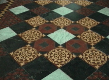
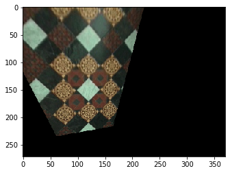
As we see, the squares have straightened out. Specifically, the correspondences have been defined only on four points with the middle diamond as reference points.

Rectification: Chinatown

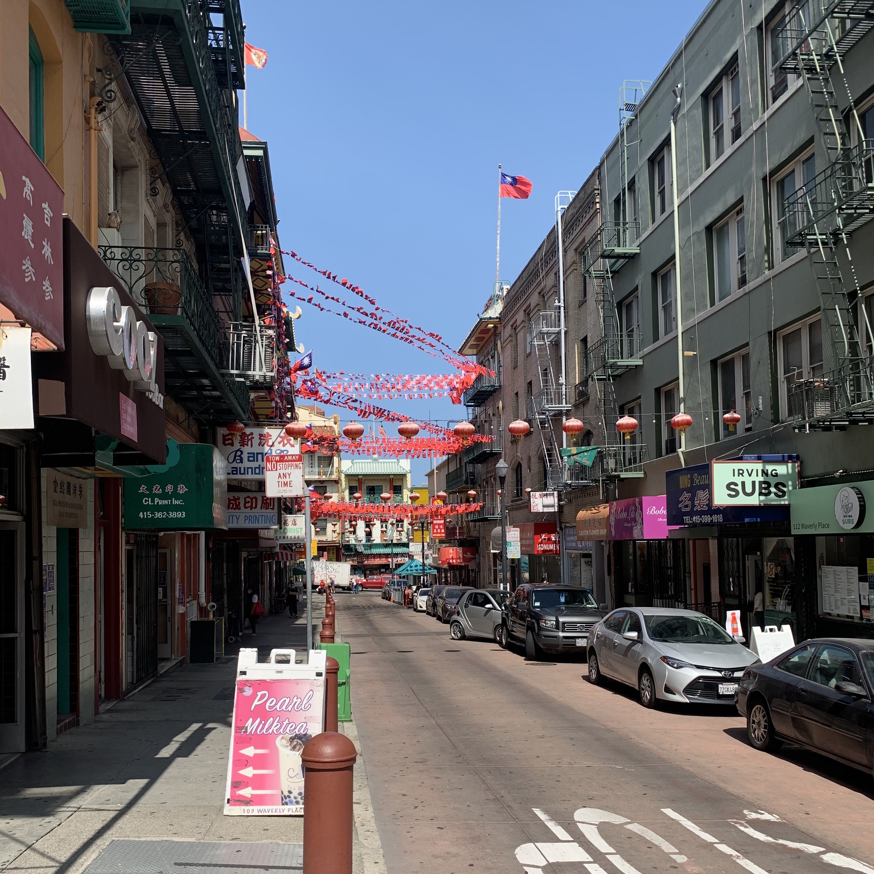
This picture was taken by me in San Francisco Chinatown from the sidewalk. As we can see, the picture on the right seems more like we are standing in front of the middle building than on the side. Nonetheless, some problems that I experienced with rectifying the picture is finding clear correspondence points that I can properly map and locate. In the previous case, it was easy to define the corresponding coordinates for a square. In this situation, I had to use only the building on the background for correspondence. I also had to guess the approximate ratio and height/width. Therefore, the result turned out particularly wobbly. Nonetheless, you still can see the effect particularly well.

Panorama

The panorama picture consisted of three individually taken pictures at soda shown above. The methodology is to assume the center image's projection to be truthful. Additionally, for warping, we would always warp to this center of truth. That means that the destination would always be in the dimension of picture 2. The source images would be image 1 and 3. Specifically, I had defined 15 correspondences, points that are overlap between the left-middle and right-middle pictures. This was particularly easy since there are a lot of geometric lines in the architecture around soda halls, as we can see in the definition of correspondences below.

After defining the correspondences, performing homographies and warping. It was important to extend the range of the pictures. I had to make the images three times as wide, so it was easier to add them to each other. After that, I performed a linear blending of where a mask would indicate that the two images would overlap. This resulted in the following panorama picture below. Something interesting is to see that the alignment is not 100% perfect which makes sense since it is done by humans. Additionally, using multiresolutional blending would not prove useful for this situation, since the problem here seems to be specifically, the coloration. A specific culprit could be the different angles of the sun that produce different amounts of lighting for the different parts of the picture.