Stitching Photo Mosaics
By Jay Shenoy
Part A: Image Warping and Mosaicing
Step 1: Shooting the Photographs
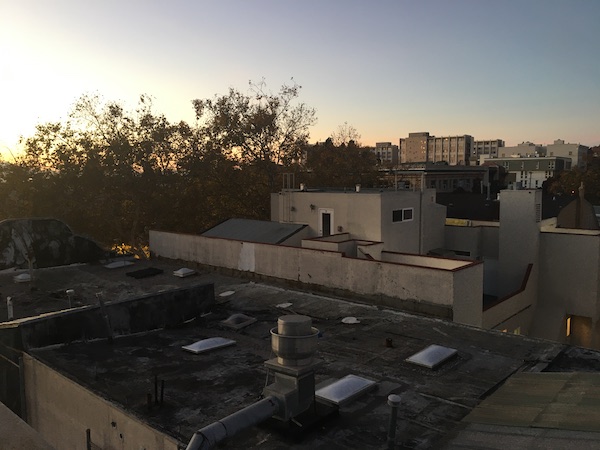
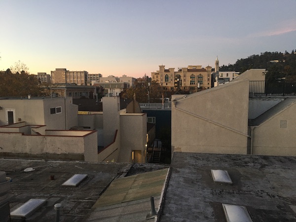
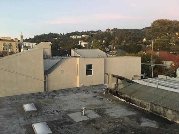
I shot three photos of the Berkeley skyline:
Step 2: Recover Homographies
I selected 12 corresponding keypoints for each pair of contiguous photographs. Here are the keypoints I selected for the images:
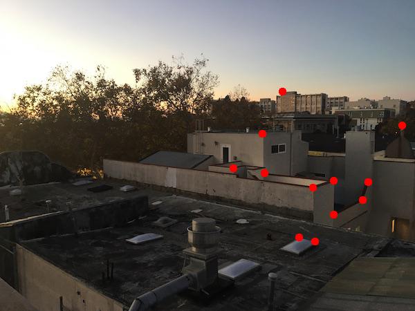 Image 1 Keypoints
|
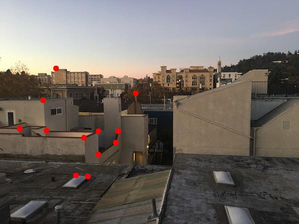 Image 2 Keypoints
|
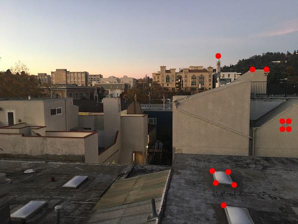 Image 2 Keypoints
|
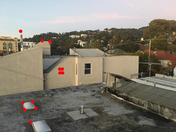 Image 3 Keypoints
|
To recover the homography matrix between these two sets of keypoints, I solved the following system of linear equations using least-squares:
\(
\begin{bmatrix}
x_1 & y_1 & 1 & 0 & 0 & 0 & -x_1 x_2 & -y_1 x_2 \\
0 & 0 & 0 & x_1 & y_1 & 1 & -x_1 y_2 & -y_1 y_2 \\
& & & & \vdots \\
\end{bmatrix}
h =
\begin{bmatrix}
x_2 \\
y_2 \\
\vdots
\end{bmatrix}
\)
Here, \( (x_1, y_1) \) and \( (x_2, y_2) \) are corresponding keypoints from images 1 and 2, respectively, and there are 6 such correspondences. Least-squares lets you solve for the vector \( h \) that minimizes the squared error. \( h \) contains 8 entries that correspond to the first 8 entries of the homography matrix (the last entry is set to one).
Step 3: Warp the Images
Homography matrix in hand, I now warped image 1 to align properly with image 2. I did this using inverse warping: for each pixel in the warped image, I determined the source pixel in the original image and used interpolation to retrieve the proper pixel intensity. Image 1 was warped to align with image 2, and image 2 was translated to fit within a larger canvas (so that both images could be overlayed).
To prove that warping was working correctly, I performed image rectification, a process that takes a portion of the image that is known to be rectangular and "rectifies" it by computing the appropriate homography matrix that will make the sides of the rectangle axis-aligned so it looks like we're observing that portion top-down. Three examples of image rectification are shown below:
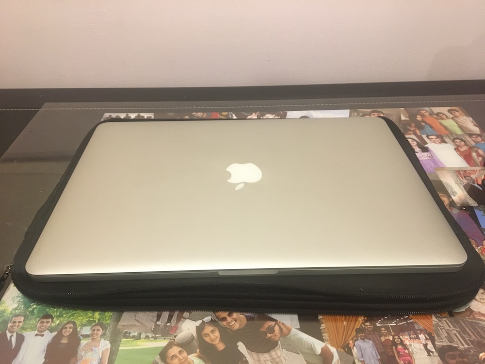 MacBook Pro Original
|
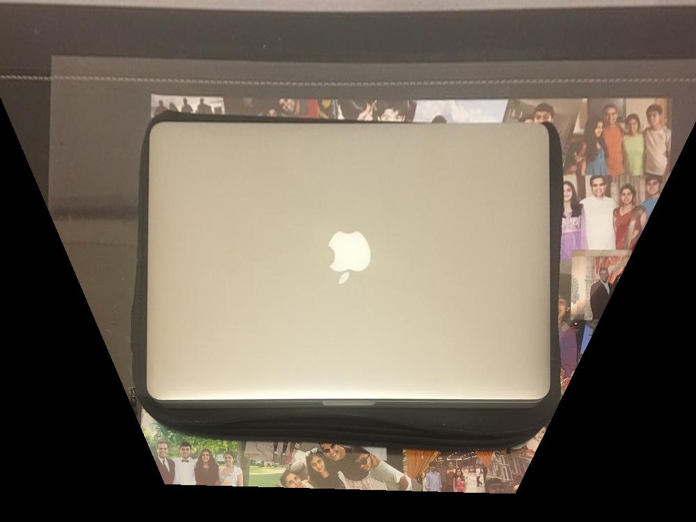 MacBook Pro Rectified
|
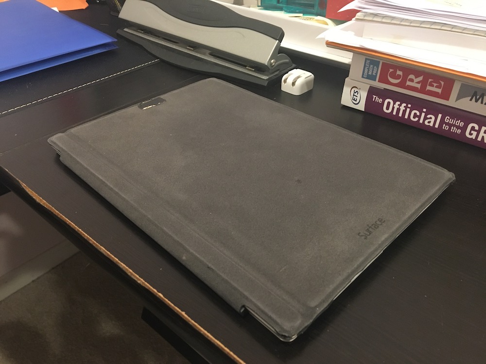 Surface Pro Original
|
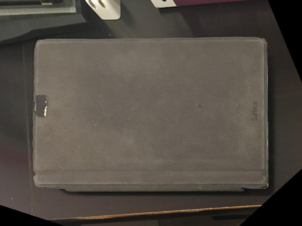 Surface Pro Rectified
|
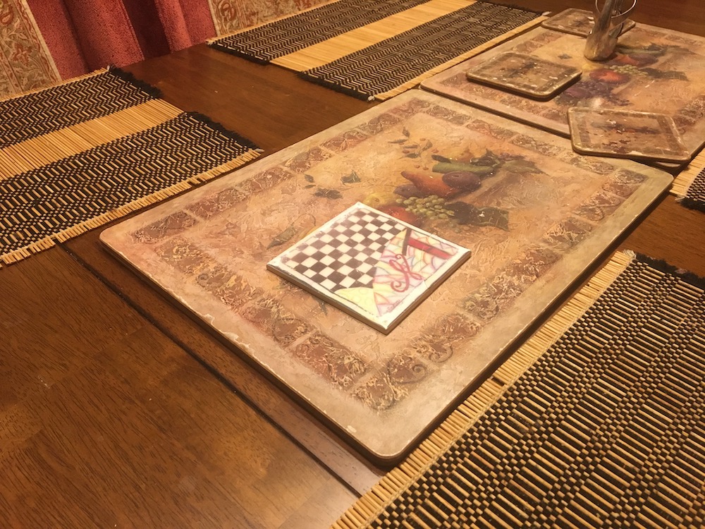 Coaster Original
|
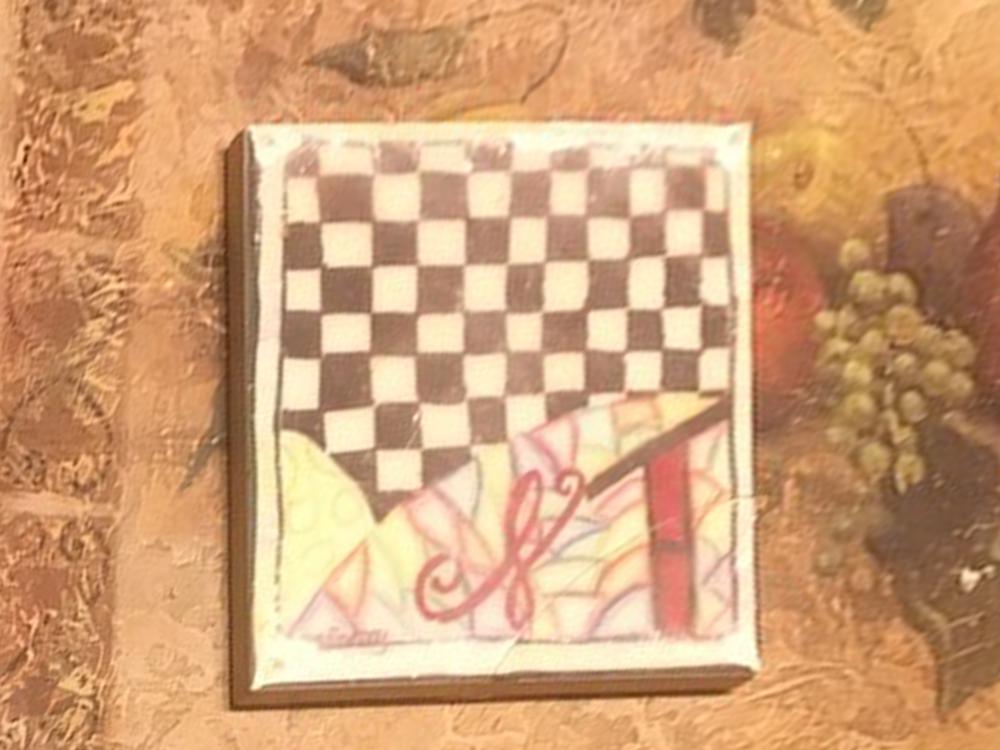 Coaster Rectified
|
Step 4: Blending
Blending the images into a mosaic is a multi-stage process. First, I warped the images into a larger canvas using the estimated homographies as described in step 3. The warped images are shown below:
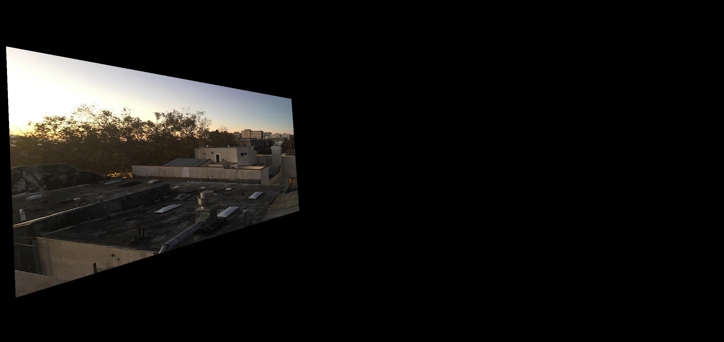 Image 1 Warped
|
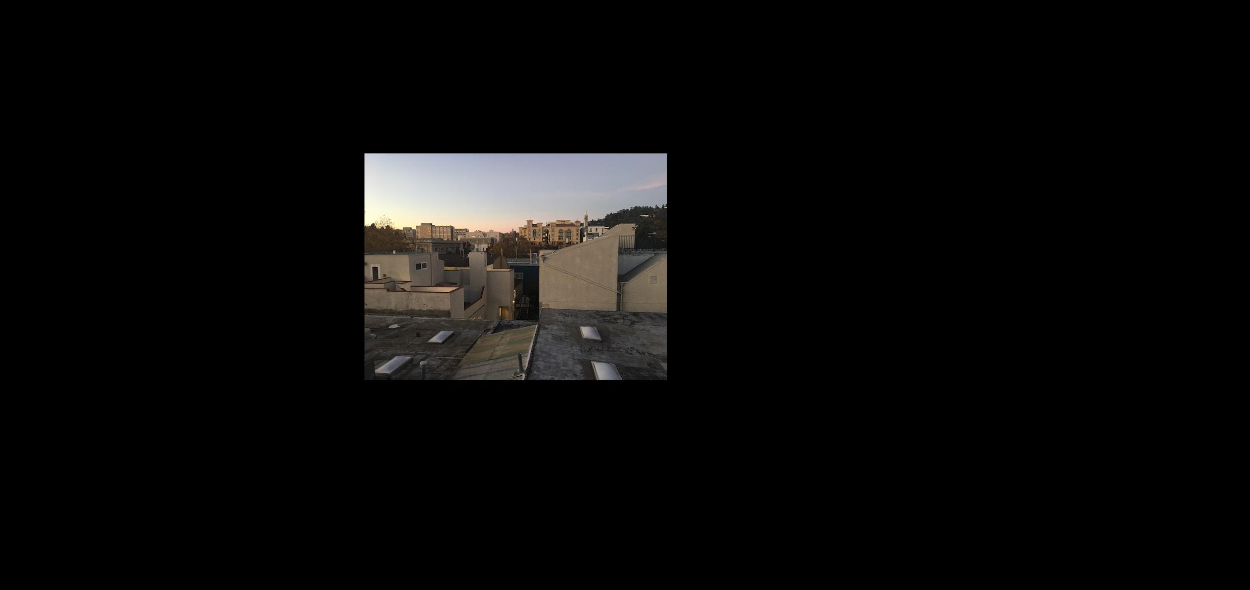 Image 2 Warped
|
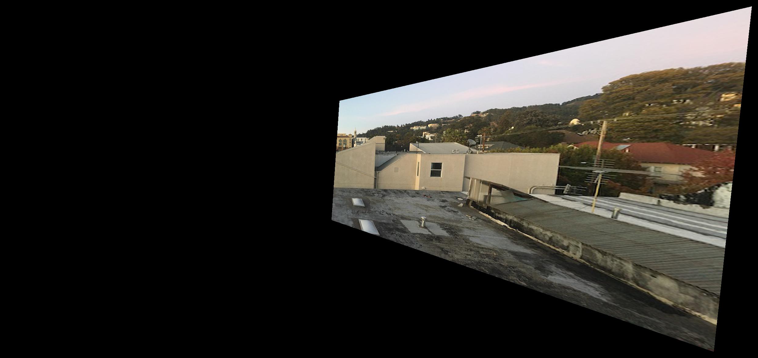 Image 3 Warped
|
To properly mosaic the warped images, I used a one-shot procedure that computed alpha weights for each pixel in each warped image. These alpha weights range from zero to one, indicating how much to feather each pixel value. The specific weights were computed linearly by setting the alphas to one at the centers of the unwarped images and having them decline to zero at the left and right edges. Below, you can see the alpha-feathered images.
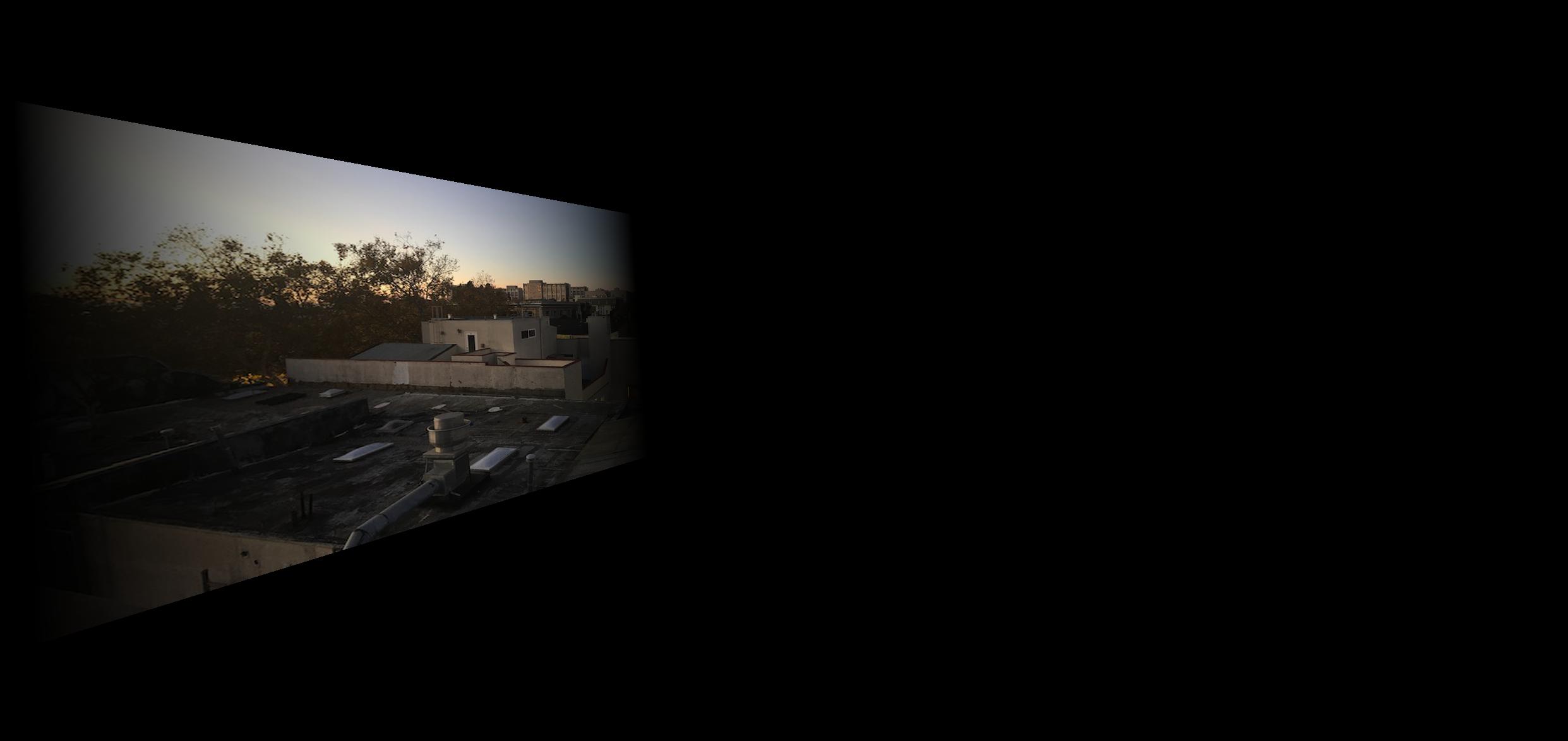 Image 1 Warped + Feathered
|
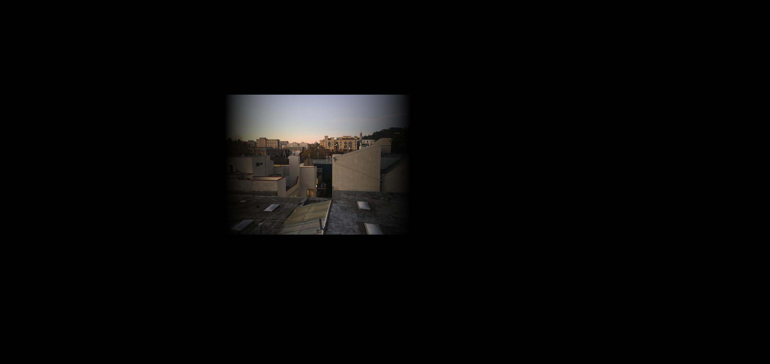 Image 2 Warped + Feathered
|
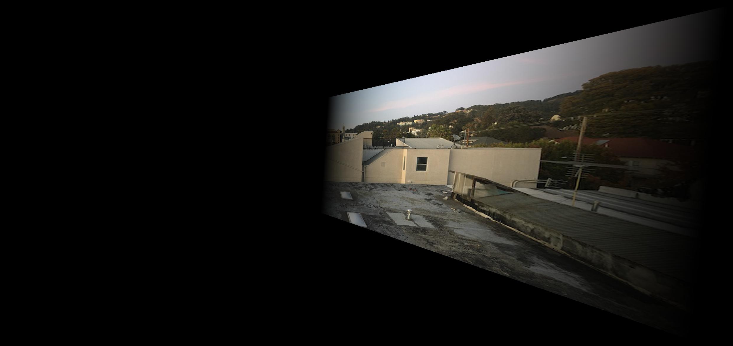 Image 3 Warped + Feathered
|
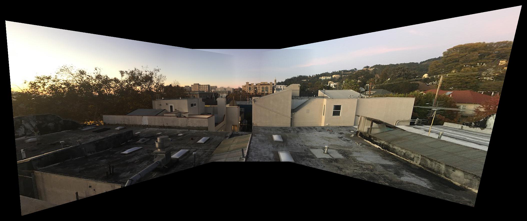
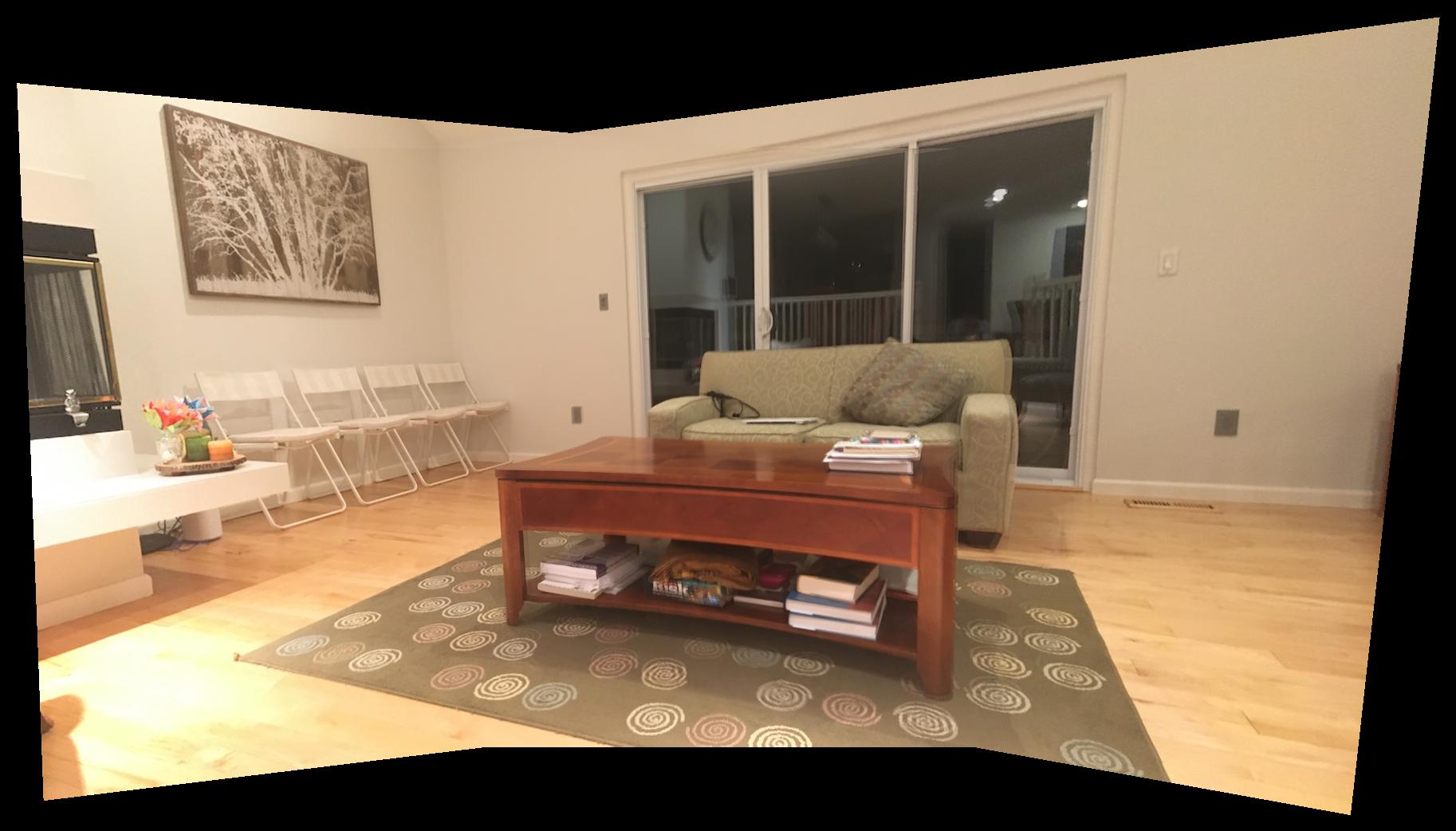
To combine these feathered images into a mosaic, I simply ensured that the alpha weights for each pixel summed to one (to get rid of any vignetting) except, of course, for pixels with no image data. The source images and final stitch are shown below for 3 examples.
 Balcony Image 1
|
 Balcony Image 2
|
 Balcony Image 3
|
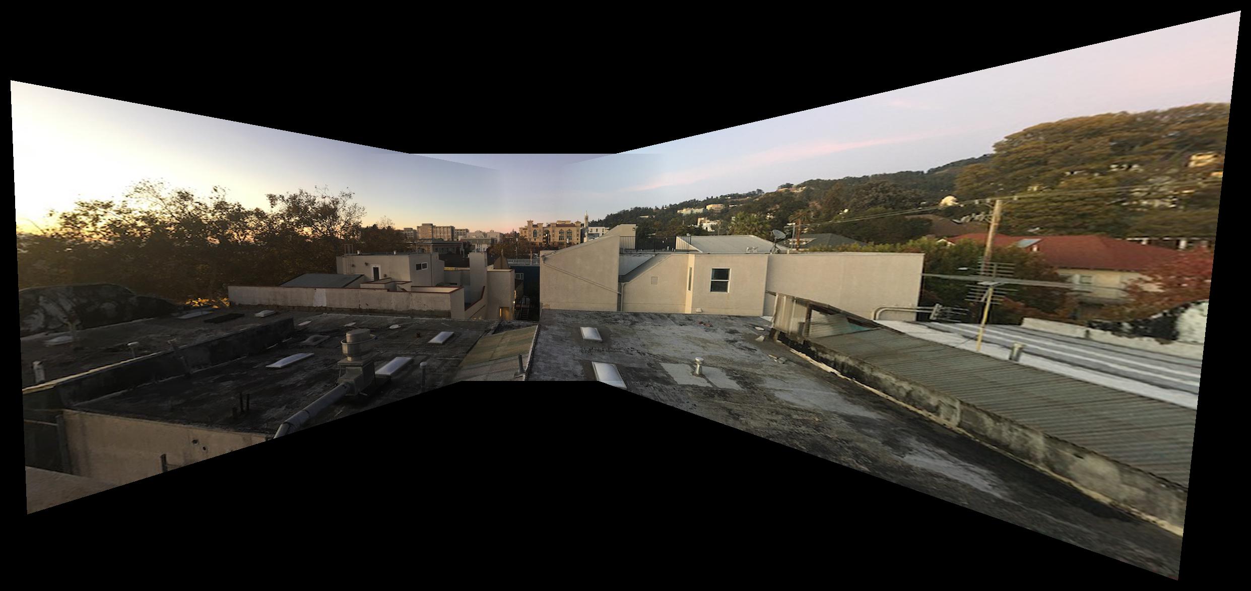 Balcony Mosaic
|
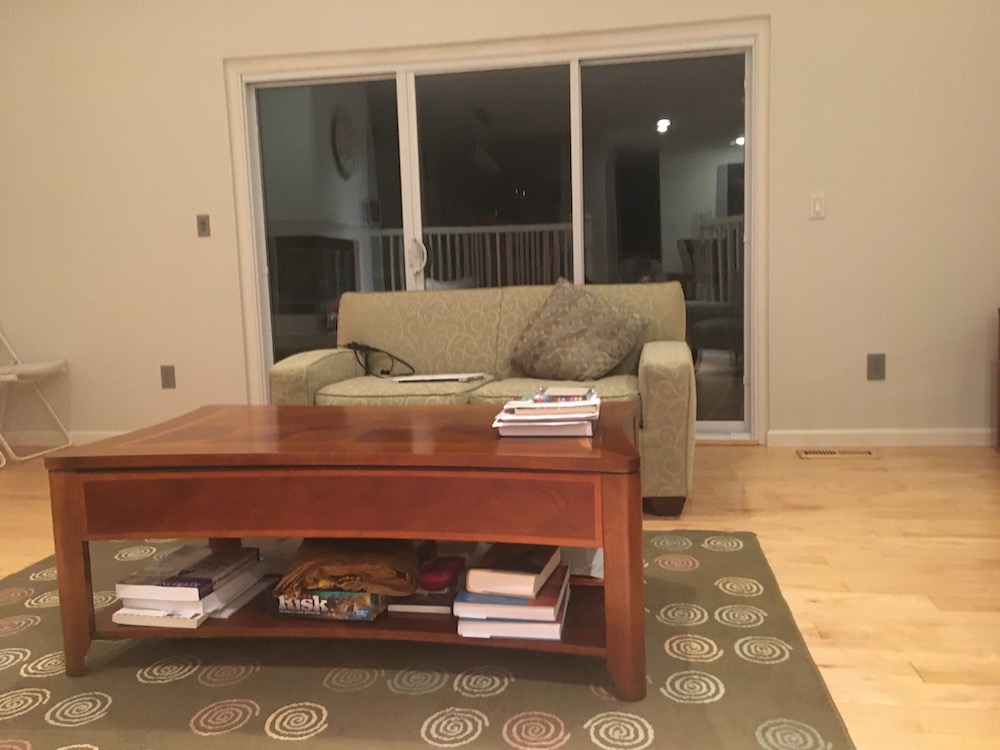 Living Room Image 1
|
 Living Room Image 2
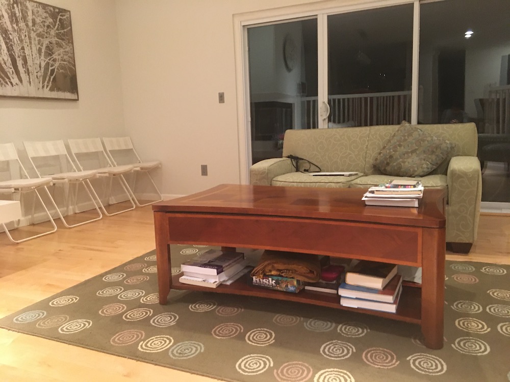
|
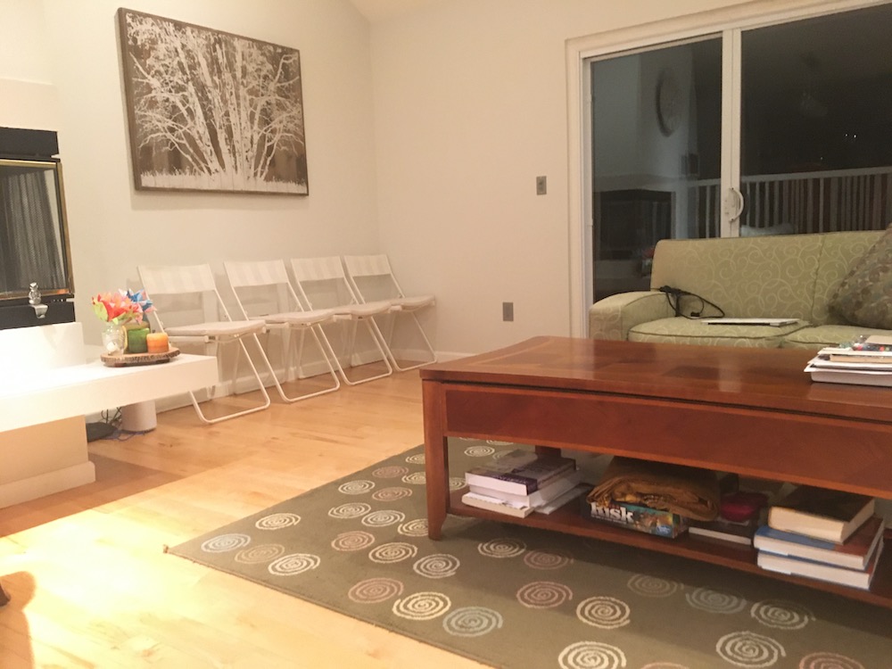 Living Room Image 3
|
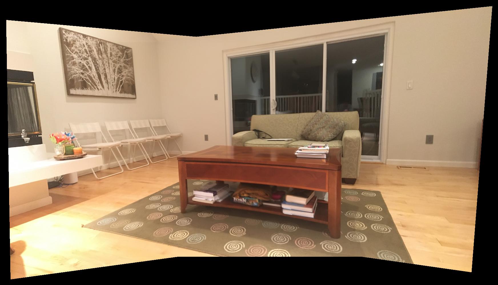 Living Room Mosaic
|
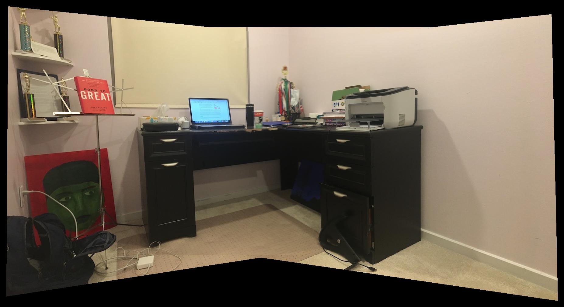
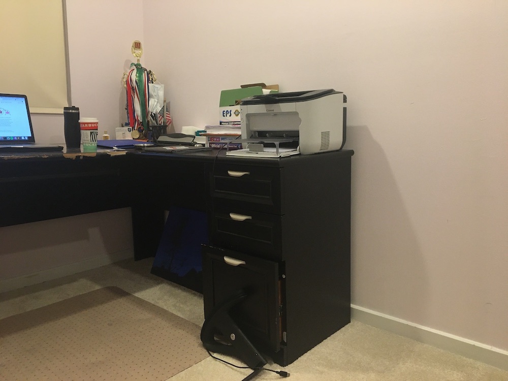 Desk Image 1
|
 Desk Image 2
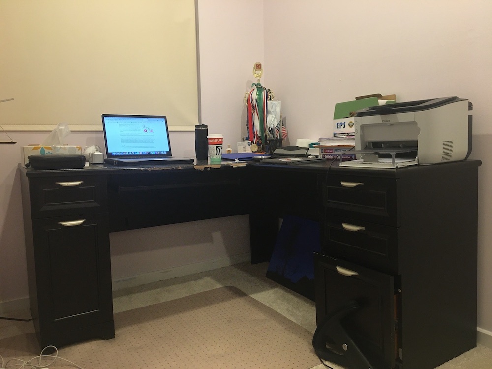
|
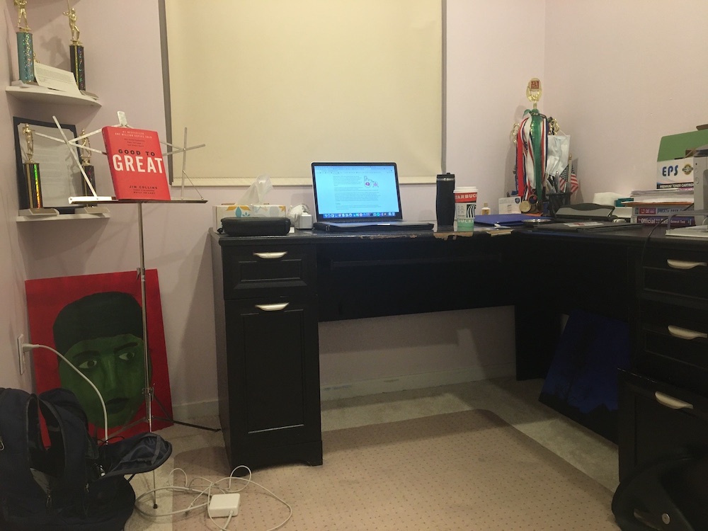 Desk Image 3
|
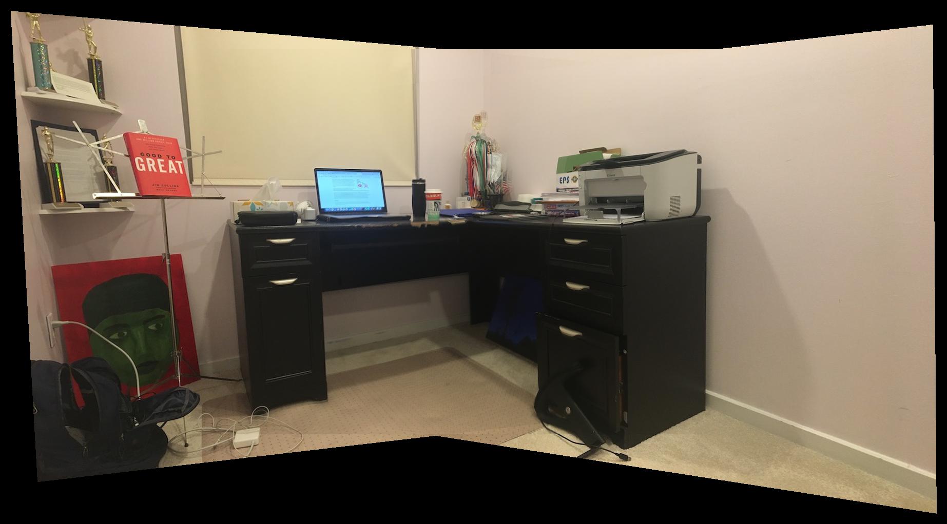 Desk Mosaic
|
What I've Learned
The coolest concept from this part of the project was that of image rectification. It's amazing that using just a homography matrix, one can visualize what a rectangular surface would look like from a bird's-eye view. In lecture, we learned about how rectification was applied to artwork to extract tile patterns and such, so it was awesome to be able to apply it to my own photographs.
Part B: Feature Matching and for Autostitching
Choosing corresponding keypoints by hand is a laborious process. To get around this, I implemented automatic keypoint matching using a technique involving "Multi-Scale Oriented Patches" (MOPS).
Step 1: Detecting Harris Corners
Using the provided starter code, I extracted Harris corners from the following image of my desk.
|
Original Desk Image
|
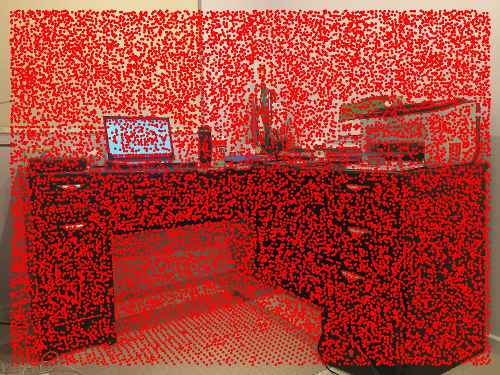 Desk with Corners
|
Next, I reduced the set of Harris corners via a technique called adaptive non-maximal suppression (ANMS). ANMS tries to pick out the corners with the highest strength (as computed by the starter code) while keeping the keypoints relatively spaced out. The ANMS procedure can be visualized as follows: create a circle at every keypoint, initially of radius zero. Now expand all the radii simultaneously: if two circles intersect, remove the keypoint with the lower corner strength. The radius at which a keypoint is removed is called its "suppression radius," and by growing the radii in this manner, we cull the set of keypoints to produce a smaller set that is both spaced out nicely and contains corners of high strength. Computing the suppression radius of the i-th keypoint is formulated as the following optimization problem:
\(
r_i = min_j ||x_i - x_j||
s.t.
f(x_i) < 0.9 * f(x_j)
\)
Here, \( x_i \) represents the position of the i-th keypoint, and \( f(x_i) \) represents its corner strength. I chose to keep the keypoints with the top 500 suppression radii. The ANMS corners are visualized below.
|
Desk with Corners
|
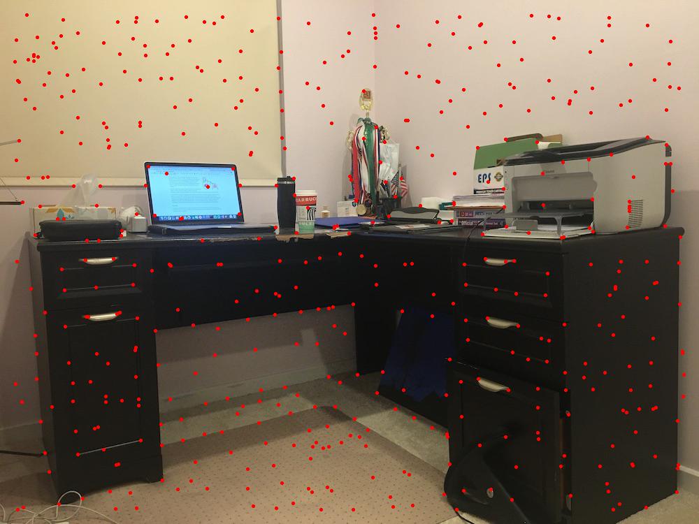 Desk with ANMS Corners
|
Steps 2-4: Extracting Features + RANSAC
After retrieving the 500 ANMS keypoints, I extracted a 40x40 image patch around each keypoint. I then downsampled this patch to be of dimensions 8x8 using a box blur. These 8x8 feature descriptors were then bias/gain-normalized so their means were zero and standard deviations were one. Next, I matched the descriptors using Lowe thresholding: for each descriptor in image 1, I computed the ratio between the distance to its first nearest neighbor and second nearest neighbor in image 2. I used a threshold of 0.25, so only (first nearest neighbor) matches below this threshold were kept.
After the feature descriptors between the two images were matched up, I used 4-point RANSAC to calculate a robust homography estimate to represent the transform between the images. The RANSAC algorithm goes as follows: first, randomly select 4 matched points, compute the exact homography between them, and determine how many of the remaining matched points are "inliers" within this homography (whose transform error is at most 2 pixels in any dimension). I ran this 10,000 times and kept the homography that had the largest number of inliers, using least-squares at the very end to create a new homography using all the inlier points.
Step 5: Mosaicing
The matched keypoints from the previous step were fed into the stitching algorithm from part 1 to create large mosaics. The manually-stitched and automatically-stitched mosaics are compared below.
|
Balcony Image 1
|
Balcony Image 2
|
Balcony Image 3
|
|
Balcony Manual Mosaic
|
 Balcony Automatic Mosaic
|
|
Living Room Image 1
|
Living Room Image 2
|
Living Room Image 3
|
|
Living Room Manual Mosaic
|
 Living Room Automatic Mosaic
|
|
Desk Image 1
|
Desk Image 2
|
Desk Image 3
|
|
Desk Manual Mosaic
|
 Desk Automatic Mosaic
|
What Have I Learned?
The coolest part about this project was implementing adaptive non-maximal suppression. I liked how the problem of finding a set of nicely-spaced keypoints of high strength was first phrased as a geometric problem involving circles centered at each keypoint that grow in size until more and more keypoints are eliminated. This offered visual intuition that helped me understand what the solution was going for. Moreover, I appreciated how this intuition was translated to an optimization problem that was relatively easy to solve, and produced great results. As shown in the images above, I thought it was impressive how the algorithm was able to cull a dense set of thousands of Harris corners down to a set of 500 keypoints that were well-spaced out.