Project 5 : (Auto)sticthing and photo mosaics

In this project, we will be combining everything that we learned in this semester through working on Mosaics. Specifically, the first part will be about implementing manual stitching. The second part will be about creating an algorithm that performs stitching automatically.

Part A: Image Warping and Mosaicing

This project can basically be divided into four main parts:

1. Data Collection
2. Homography Recovering
3. Inverse Warping and Rectifications
4. Panorama: Blending mosaic

1 - Data Collection

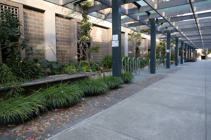
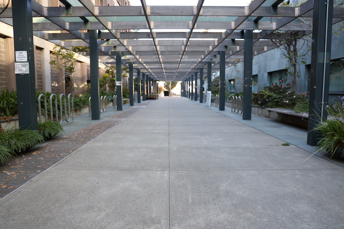
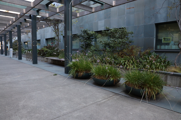
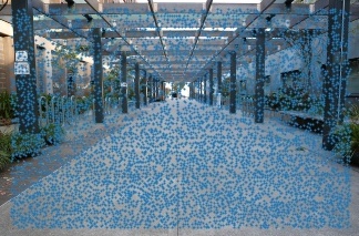
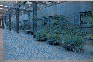
For the purpose of this project, I took out my mirrorless camera and started thinking about where to take picture. I wanted a place that had a lot of features that I could create correspondences on. Additionaly, I wanted to pick a place that has a lot of significance to me. Therefore, I decided to take a series of pictures on a triped with my mirrorless camera in front of Soda Hall, the home of the Computer Science Department at Berkeley. The pictures can be seen below.

But I also realized that the state of California reinstated the Shelter in Place orders, so the other set of pictures are less spectacular, namely my home.

Since these pictures are gigantic, however, I have decided that I will only be using 10% of their original resolution.

2 - Homography Recovery

For a homographic projection, we normally only need 4 2D coordinates to define the transformation matrix (since there are only 8 degrees of freedom). However, as we defined in class, it's better to create an overdetermined system to solve for the homography matrix in order to decrease the effect of noise. For overdetermined systems, however, we are required to solve it through least squares. Specifically, we can derive the following identity: $$\hat{w} = (X^{T}X)^{-1} X^{T}b$$

Nonetheless, we still need to create some restrictions to force the solution to give us an output of 9 variables (or also in this situation 8, since we know there are 8 degrees of freedom). Specifically, we want to find $$^{argmin}_{ H} H p - p'$$. Equivalently, we want Hp (transformations of H on our original points p) to be as close as possible to our destination points p'.. One way to go around this is to construct p into the form of a 2n by 8 matrix. Then we flatten b and complete this matrix p in such a manner that we can recover the homography. At the end of the recovery of the 8 parameters, we can reshape it and add a 1 at the end as the normalization factor.

3 - Warping and Rectification

I created a warp function through using the cv2.remap function. The way to construct the function remap is first by taking the inverse of our homography projection matrix, since we will be performing an inverse warp. After that, you initiliaze a matrix that indicates its x and y coordinates in the same shape as the original image. After that, we flatten these matrices and mold them into the shape of p where one column is [x,y,1].T. This representation is basically all the points that exist in our destination picture. Then we inverse warp it and multiply this by the former, we gain the resulting coordinates of where the source pixels reside. cv2.remap takes care of the interpolation and lookup of these pixels.

Combining these results from 2 and 3, gives us the following rectifications:

Rectification: Pattern

As we see, the squares have straightened out. Specifically, the correspondences have been defined only on four points with the middle diamond as reference points.

Rectification: Chinatown

This picture was taken by me in San Francisco Chinatown from the sidewalk. As we can see, the picture on the right seems more like we are standing in front of the middle building than on the side. Nonetheless, some problems that I experienced with rectifying the picture is finding clear correspondence points that I can properly map and locate. In the previous case, it was easy to define the corresponding coordinates for a square. In this situation, I had to use only the building on the background for correspondence. I also had to guess the approximate ratio and height/width. Therefore, the result turned out particularly wobbly. Nonetheless, you still can see the effect particularly well.

Panorama

The panorama picture consisted of three individually taken pictures at soda shown above. The methodology is to assume the center image's projection to be truthful. Additionally, for warping, we would always warp to this center of truth. That means that the destination would always be in the dimension of picture 2. The source images would be image 1 and 3. Specifically, I had defined 15 correspondences, points that are overlap between the left-middle and right-middle pictures. This was particularly easy since there are a lot of geometric lines in the architecture around soda halls, as we can see in the definition of correspondences below.

After defining the correspondences, performing homographies and warping. It was important to extend the range of the pictures. I had to make the images three times as wide, so it was easier to add them to each other. After that, I performed a multiresolution blending at the area where the pictures would intersect - 50, since otherwise we would see weird black artefacts. As can be seen below, the blend is seamless, but the color is not entirely right which is quite odd since I used the same manual settings on my camera. It might have been the weird light situation during that time of the day which caused the three pictures to have different lighting which makes the picture not super perfect. Nonetheless, the alignment is not bad.

I did the same thing for the corner pictures in my house. This one turned out really well since the lighting was identical. The stitching for this one looks much better! With even only 5 correspondences!

End Part A: Lessons Learned

I have to say that I never thought about how painful the process is of creating homographies when you have to do it manually. Also, the consequences of using least squares (without any type of outlier rejection) is extremely important as we can see that one outlier can screw up the complete homography. Nonetheless, it was not that painful after all, very inefficient. Therefore, we will be performing automatic correspondence alignment in the next section to which I am pretty much looking forward to.

Part B: Autostitching

In this part of the project, we are tasked to abandon the manual correspondence input through a series of smart implementations (without using ML!), following Multi-Image Matching using Multi-Scale Oriented Patches” by Brown et al. After the correspondence, we blend it and warp it in a similar fashion as we did in part A. An basic struture on how to perform autostitching:

1. Harris Interest Points Detection
2. Adaptive Non-Maximal Suppression
3. Feature Descriptors
4. Feature Matching
5. RANSAC
6. Computing Homography, Inverse Warping and Blending as in part A

B1: Harris Interest Points Detecion

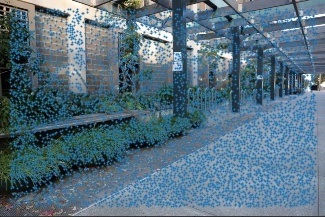
Harris Point Detection basically looks for corners through the basic property that when you zoom in on a corner and you move into any other direction, we will get a very big shift in intensity, while that's not true for lines. Through a series of linear algebra rewriting, we get to find the harris interest points through computing matrix M based on the image derivatives. The ratio of the determinant and the trace gives us the response function R. We basically take the local maxima of R and we get our harris points. The harris points are shown below for all our pictures used. We see that there so many points. This makes sense, since buildings and houses are full of corners since they are squared and therefore, we have a lot to choose from.

B2: Adaptive Non-Maximal Suppression

But, we don't need hella points! We only need a few to define a correspondence. Therefore, we will try to reduce the density of the points of interest. The objective that we are going for here is trying to get points that are spaced out as much as possible as well as having a higher 'interest' score possible. We will be using the ANMS algorithm as described in the paper. We calculate the R-score for each of the points. The points with the largest x r-scores will be taken. Here we will be going for top 500 points. The R-score is defined as: $$r_{i} = \min _{j} \|x_{i} - x_{j}\| \space s.t. \space Harrisscore(i) < 0.9 * Harrisscore(j)$$

B3: Feature Descriptors

Okay cool, so we independently selected 500 points for each image to be warped. Now we have to match these points. Before we can match, we need a summary of each of the corners such that they are invariant to noise, intensity shifts, rotations, scale, homographic projections. flatten the vector, becoming a 1x64 vector. For the purpose of panoramas, I will not be implementing scale invariance or rotation invariance.

B4: Feature Matching

Now we can match features. As discussed in class, we can just brute force search it. Nonetheless, we also need to take care of the outlier detection. Through analysis in the paper, we have to make sure that our NN algorithm picks the right point. Therefore, if the ratio between the first and second closest neighbors is lower than 0.3, it is considered as good enough! This yields the following features being matched. Pretty good! For reference, all the ANMS points are also overlaid.

B5: RANSAC

But outlier detection isn't good enough. As per part A, we found out that Least Squares is extremely sensitive to outliers. Therefore, we have to create a way to find the points that create the best homography. One way to do that is through consensus. It's kind of how democracy works. We sample a random number of points, see which one of the samples creates the majority vote. This will help us to reject the outliers. One way to measure if points are correct is through putting a threshold. If the RMSE is larger than 3, we can say that they don't agree with the proposed homography. This creates extremely robust homographies, but it might take a little longer if you did not optimize for that work.

B6: Compare Results

By using the same warping and blending as before, we get the following result! Pretty neat!

End Part B: Lessons Learned

It was extremely insightful to implement this misleadingly easy task, finding correspondences automatic. Initially, I thought we would be implementing a ML algorithm based on data that we have. Often, we don't have access to enormous amounts of data and we are confined to feature-based implementations through thorough analysis. It was extremely interesting that a lot of the implementations that we came up with such as MOPS, feature descriptors, feature matching and RANSAC themselves are built on pretty intuitive topics. Take RANSAC, it is extremely intutive to think about getting the homography to which the most points agree. Additionally, the feature desciptor and matching are pretty intuitive too. Nonetheless, some other parts, on the other side, were a little tougher. I would have never come up with the algorithm to find an evenly spread out number of points in ANMS. Harris detectors are, on the other hand, pretty interesting. All in all, it was really cool to implement this methodology and I hope that I will get the chance to do mure of this stuff in graduate school. /p>