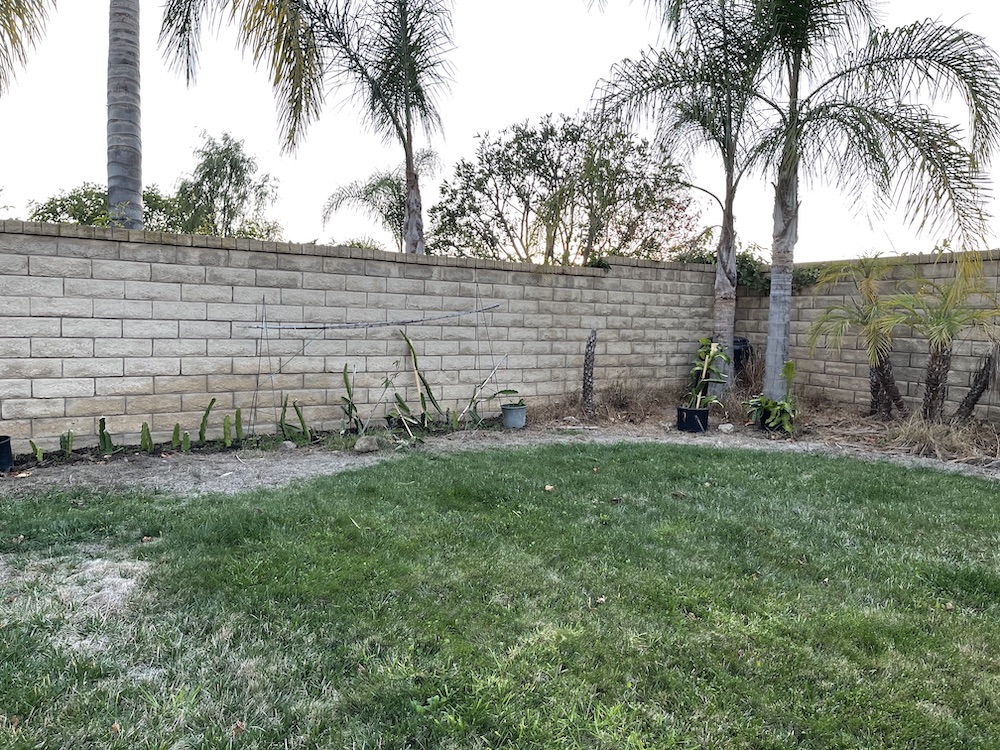
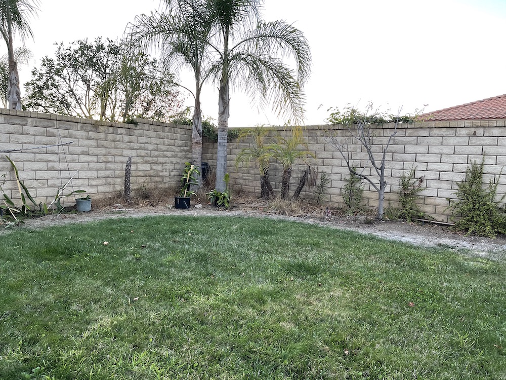
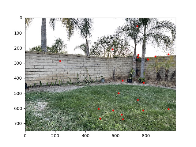
These are the pictures I took:
To recover an equation in least squares format, I did the following: $$p' = Hp$$ $$\begin{bmatrix} wx' \\ wy' \\ w \end{bmatrix} = \begin{bmatrix} a & b & c \\ d & e & f \\ g & h & 1 \end{bmatrix} \cdot \begin{bmatrix} x \\ y \\ 1 \end{bmatrix}$$ From this, we can recover two equations: $$\begin{bmatrix} a \\ b \\ c \end{bmatrix} \cdot \begin{bmatrix} x \\ y \\ 1 \end{bmatrix} = \begin{bmatrix} g \\ h \\ 1 \end{bmatrix} \cdot \begin{bmatrix} x \\ y \\ 1 \end{bmatrix} x'$$ $$\begin{bmatrix} d \\ e \\ f \end{bmatrix} \cdot \begin{bmatrix} x \\ y \\ 1 \end{bmatrix} = \begin{bmatrix} g \\ h \\ 1 \end{bmatrix} \cdot \begin{bmatrix} x \\ y \\ 1 \end{bmatrix} y'$$ Formatting this as \(Ax = b\), where \(x = \begin{bmatrix} a & b & c & d & e & f & g & h\end{bmatrix}\), $$\begin{bmatrix} 1 & 1 & 1 & 0 & 0 & 0 & xx' & yx' \\ 0 & 0 & 0 & 1 & 1 & 1 & xy' & yy' \\ \end{bmatrix} \cdot \begin{bmatrix} a \\ b \\ c \\ d \\ e \\ f \\ g \\ h \end{bmatrix} = \begin{bmatrix} x' \\ y' \end{bmatrix}$$ After stacking these for all of the selected point correspondences, I solved the linear equation with np.linalg.lstsq.
The image warping procedure is similar to project 3. I first computed the bounding box of the original image when transformed into the new plane; then sampled in the inverse direction from the original image, using RectBivariateSpline interpolation.
This is the original image:
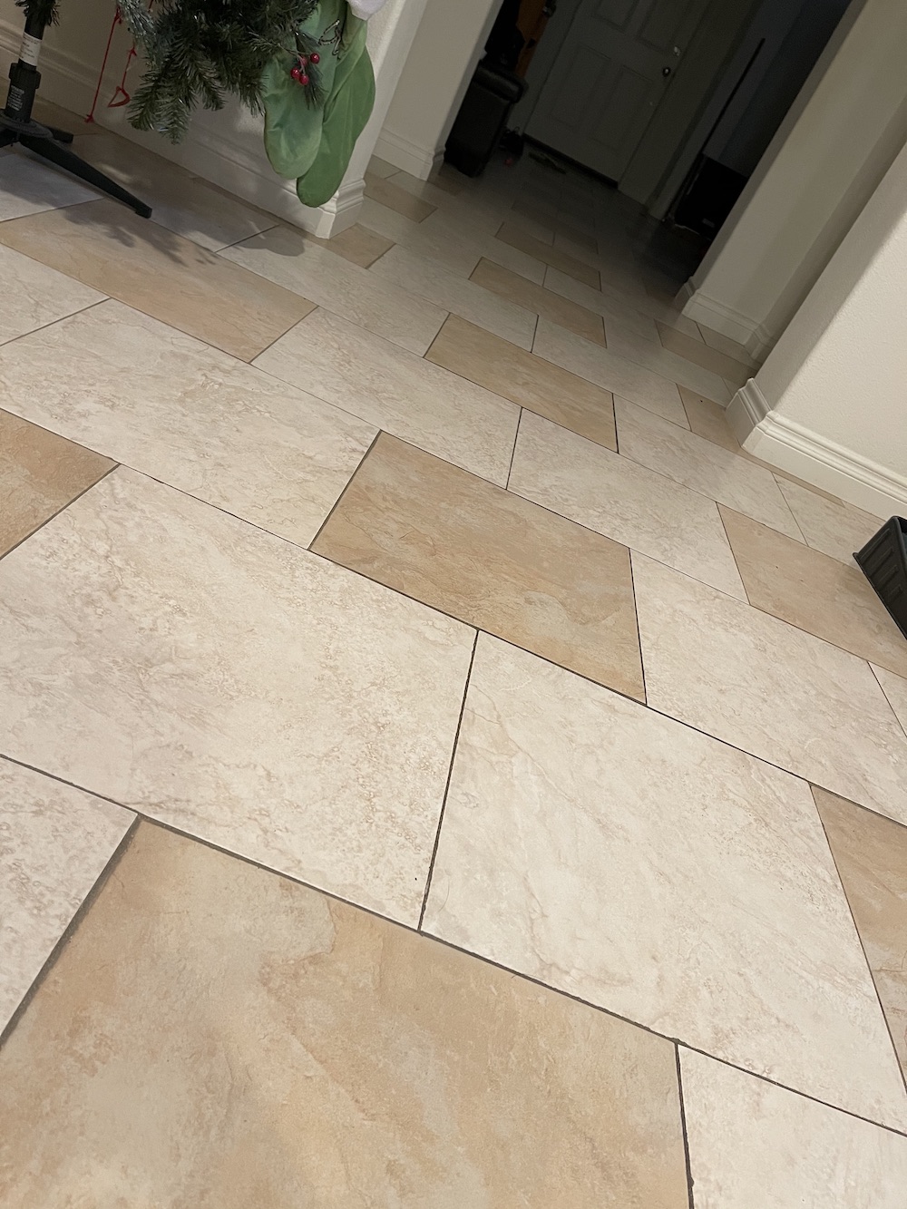
Rectifying on a floor tile as a square gives the following result:
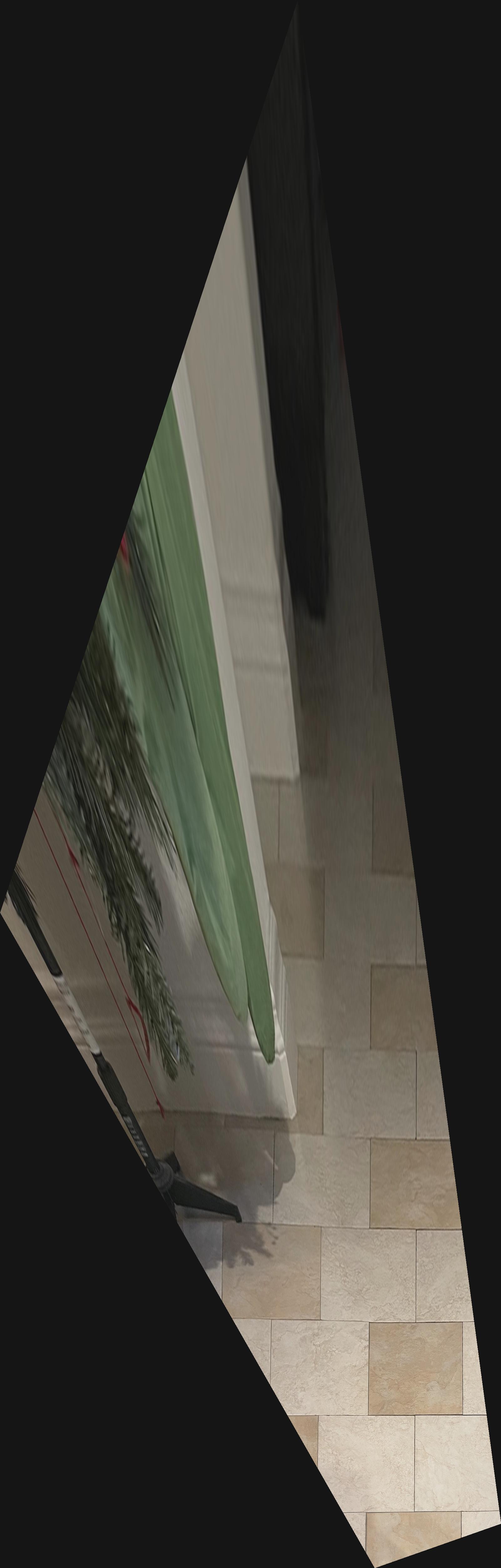
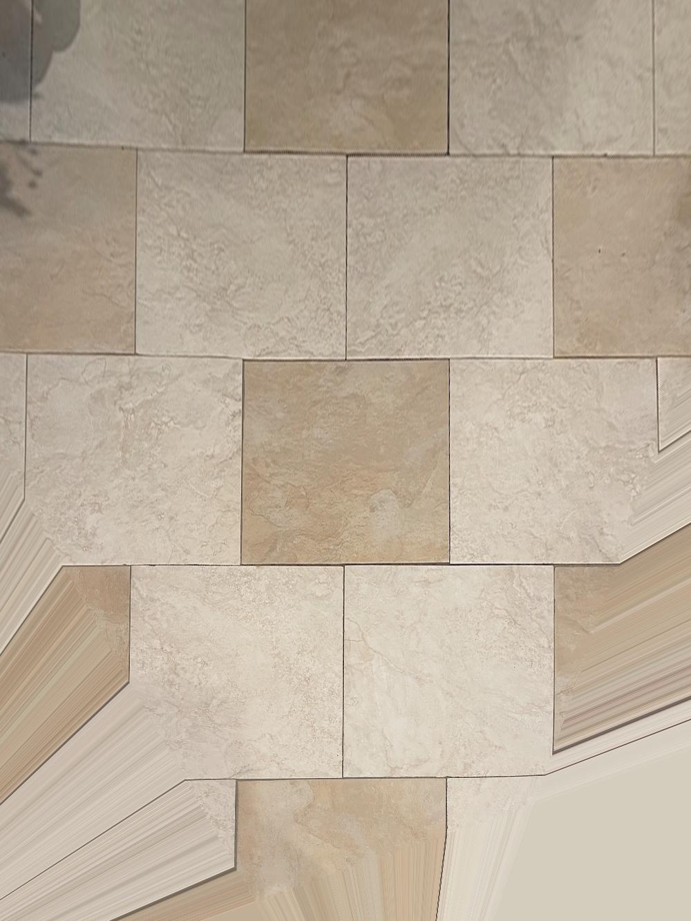
The upper right corner of this image is missing; I'm not really sure why. Depending on the selection of the square I was able to get the full image once, but was not able to reproduce.
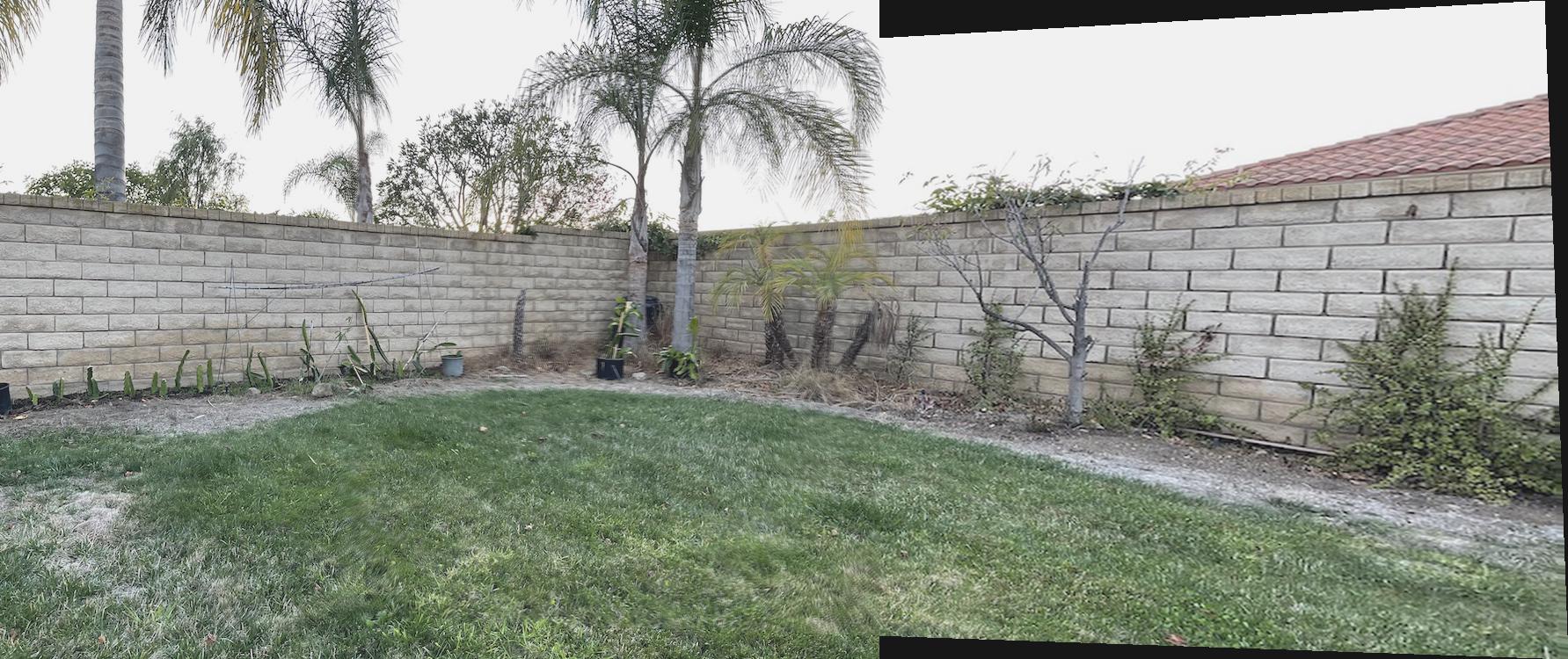
The mosaicing worked pretty well; I selected 10 correspondence points on each image, and combined them after using the resulting homography to translate the second image to the perspective of the first.
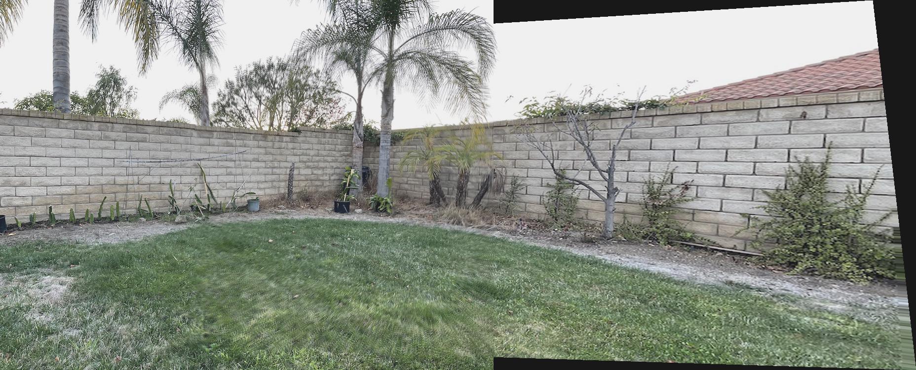
One of the seams is very slightly visible, although I'm not sure whether I'm imagining it. The overlapping parts of the image were sampled at 0.5x from each image.
The correspondence points were chosen as certain features of plants, walls, etc.
This part is based on the Multi-Image Matching using Multi-Scale Oriented Patches paper by Brown et al.
Using the same panorama images gives these results:
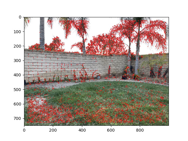
I had to make a modification of using corner_peaks instead of peak_local_max.
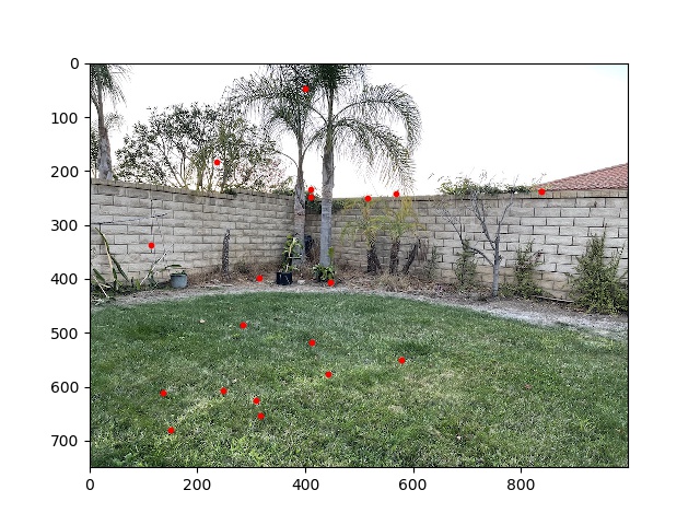
I also implemented Adaptive Non-Maximal Suppression, selecting the 500 top interest points based on radius within which their h-values were greater than 0.9 times the other h-values.
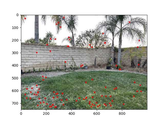
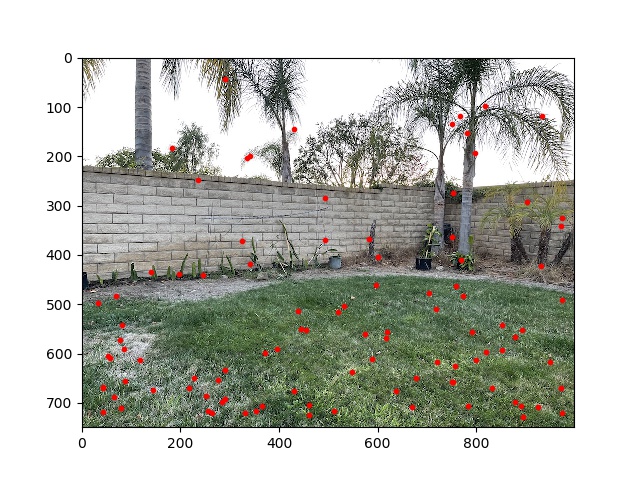
These actually look quite similar, the ANMS has some better spread on the top left but worse on the bottom left.
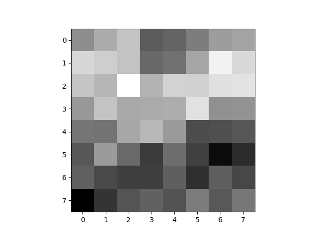
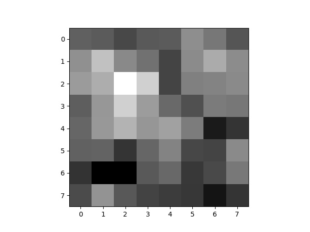
I sampled 8x8 points around each feature, with a 5 pixel spacing between samples and a 5x5 Gaussian filter applied to the whole image. These are represented as greyscale.
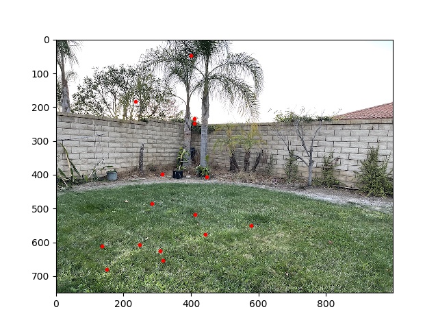
For each feature descrptor, I compared the ratio of its first and second nearest neighbors in the feature descriptors of the other image. If this was above 0.8, I kept the pair of features as matches. This resulted in the following feature points:
This looks fairly good; by inspection we can tell that there are only one or two wrong matches.
To get rid of those last couple bad matches, I implemented RANSAC. Since there are only 20 points left after Lowe's, I only iterated 5 times on the algorithm. In each iteration, I randomly chose 4 of the matches to construct a homography from; found the number of total matches that were within 5.0 pixels of each other using this homography; and returned the homography formed by the largest group of total matches across iterations.
This removed the remaining outliers:

Putting it all together, I can auto-stitch the following result, which looks pretty good and very similar to manual stitching.