Results from part A

Shooting the pictures

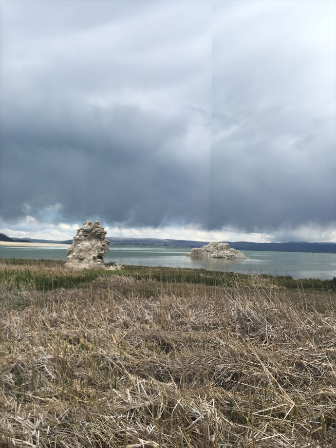
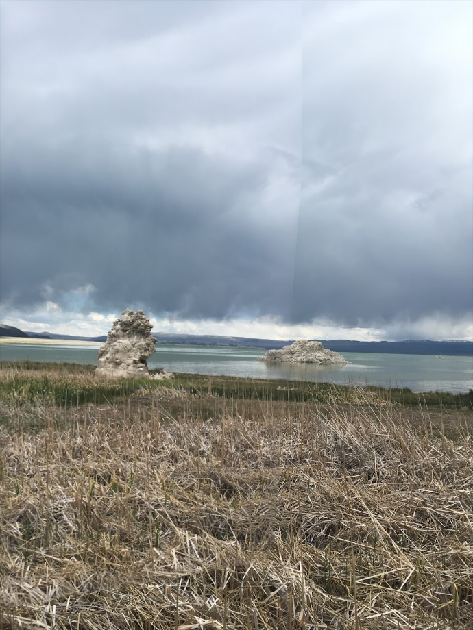
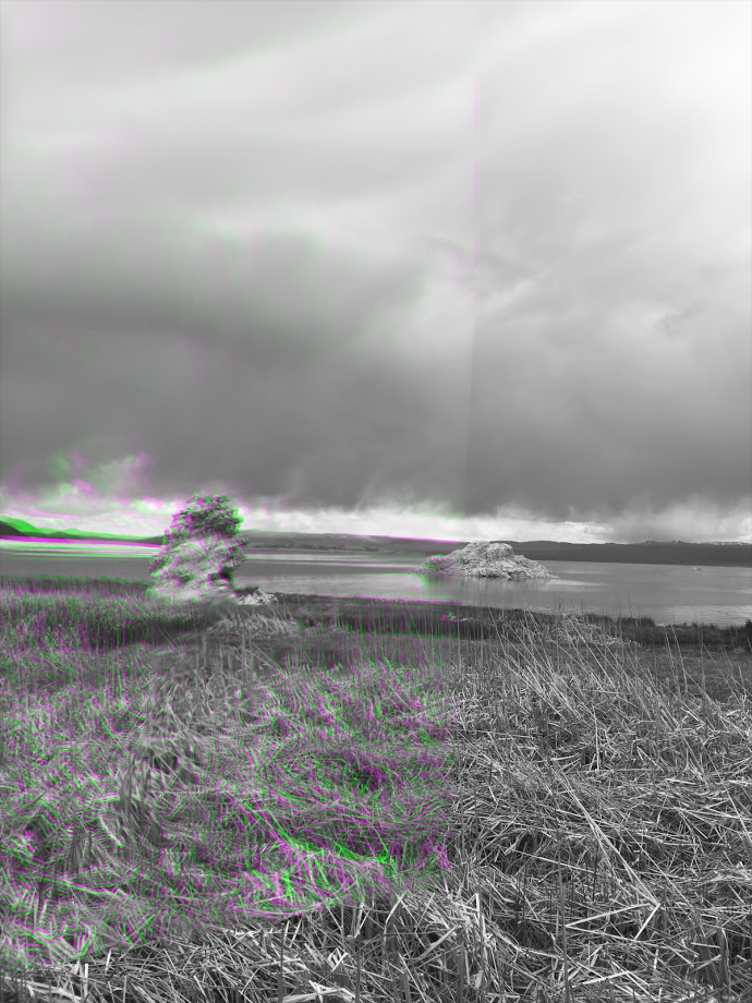
These images are a mix of new and old. I thought it would be fun to make some panoramas or mosaics of pictures I had taken on past vacations and see if I could make some warps even without conscious effort to ensure the pictures would be related by a homography. Some were impossible, and some came out pretty well!

Recovering homographies

I tried to choose pictures that represented a variety of homographies-- same points of view with different view directions, overlapping fields of view, and different shots of a scene at infinity. I handpicked points and tried the warps with and without using cpcorr. The results weren't drastically different, so I kept cpcorr just for peace of mind on picking consistent points. These points were passed into computeH which computes the homography matrix. This matrix is created by leveraging the relationship Hp = p'. Because the scale factor w is shared across the transformed p' points wx, wy, w, we can use that to write the third equation in terms of the first two, like so:

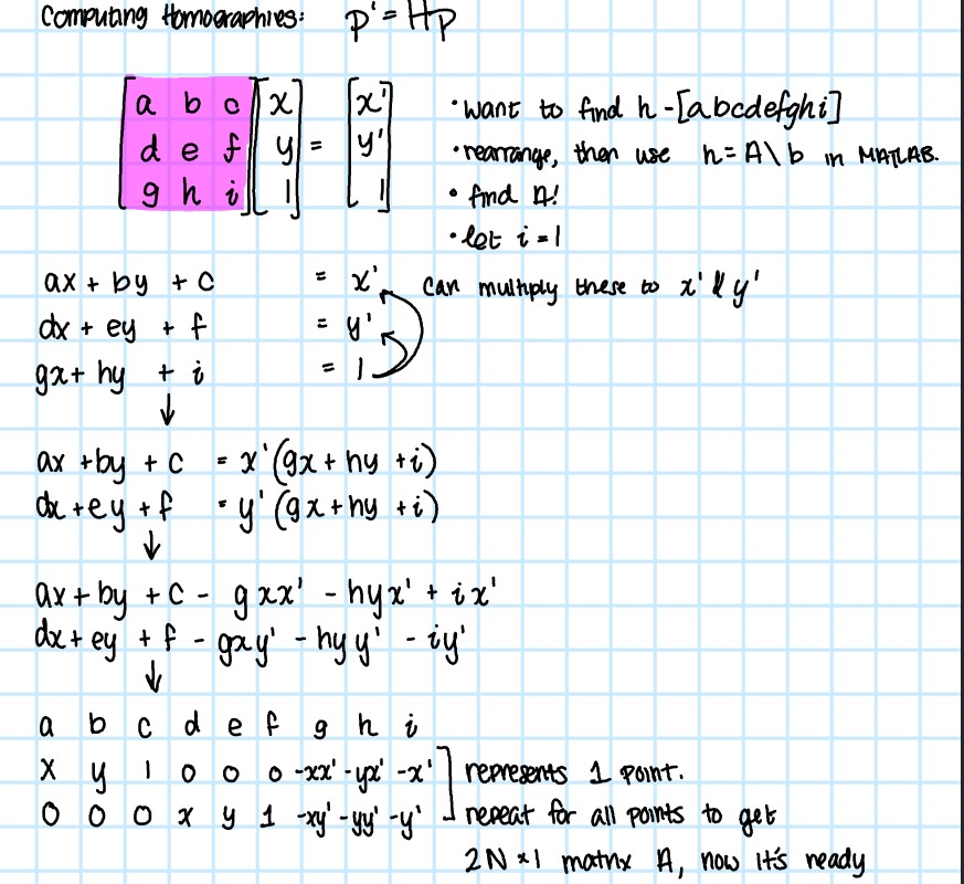
Because I used so many points to make the correspondences, I used SVD to solve the system of equations to get the a, b, c, d, e, f, g, h, i needed to reshape into the homography matrix.

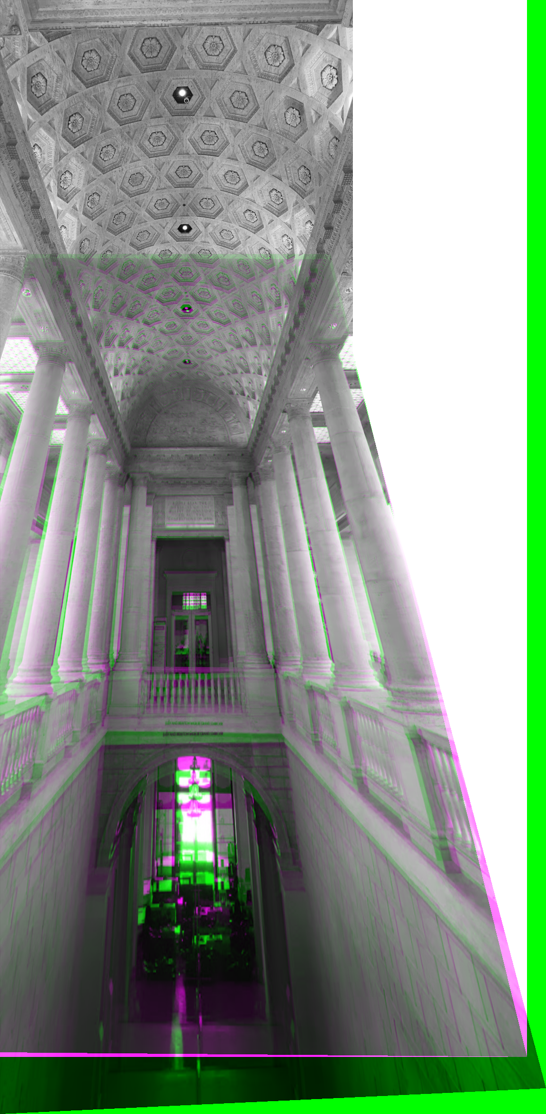
Warp the images

To warp the images, I first found the max and min of where the points in the source image would go. I then created a 'canvas' of pixel coordinates as large as the transformed height and width interpolated those pixels with an inverse H to get the color of where a transformed point came from in the original image. I also used this as a test to see whether my homography matrix was behaving as expected-- if it transformed into a very large or very small 'canvas', then I would know that these images weren't actually related by a homography, I picked bad points, or I should look over what I had done to see if the transformed points made sense.

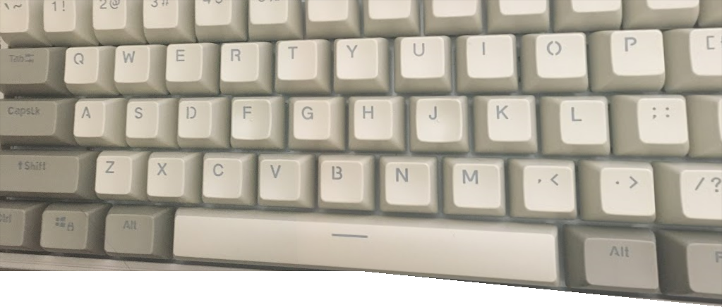
Rectification

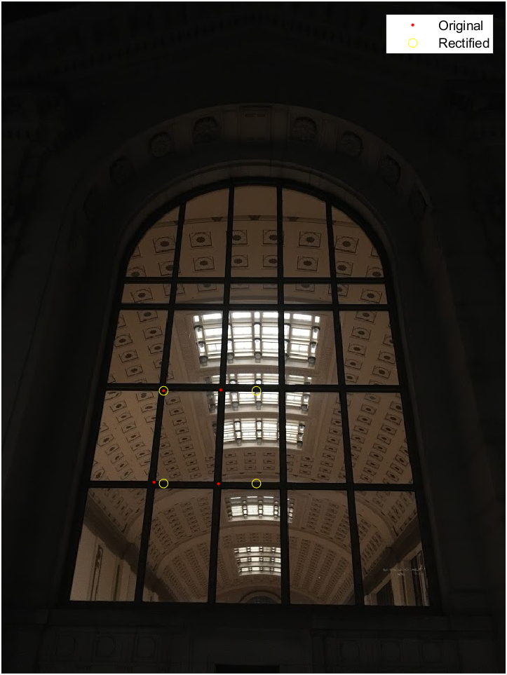
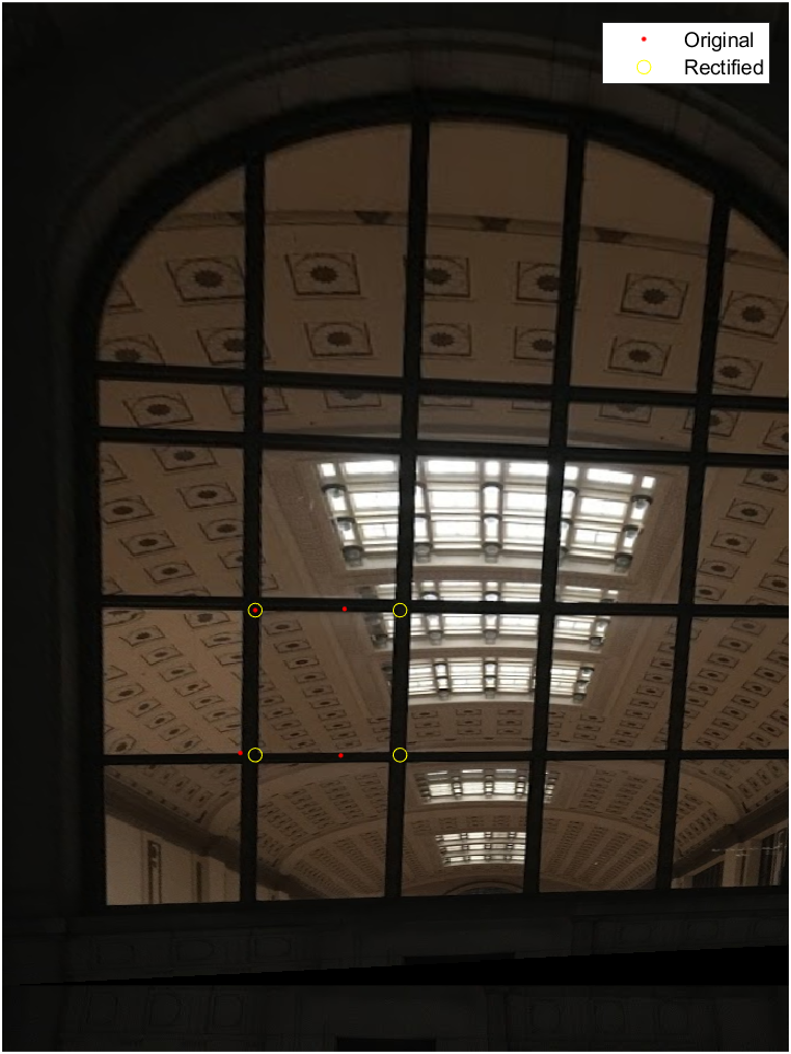
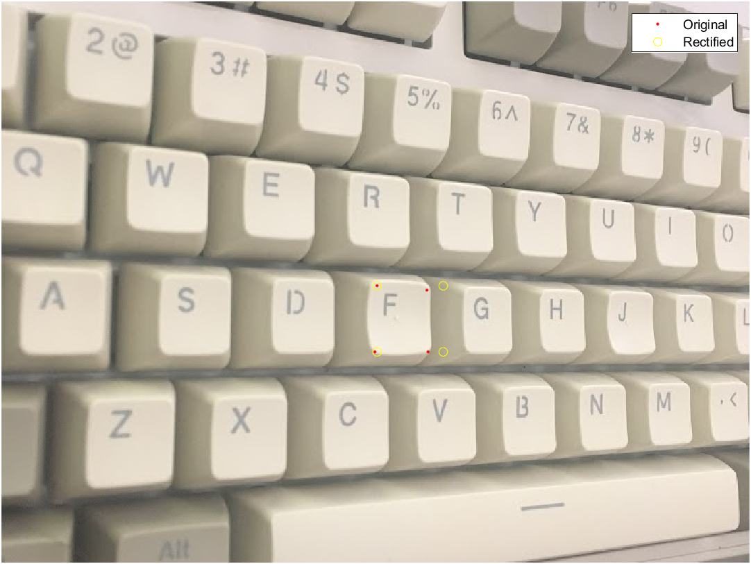
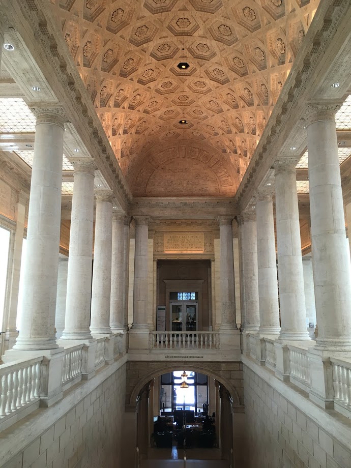
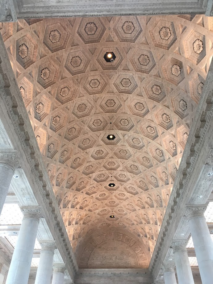
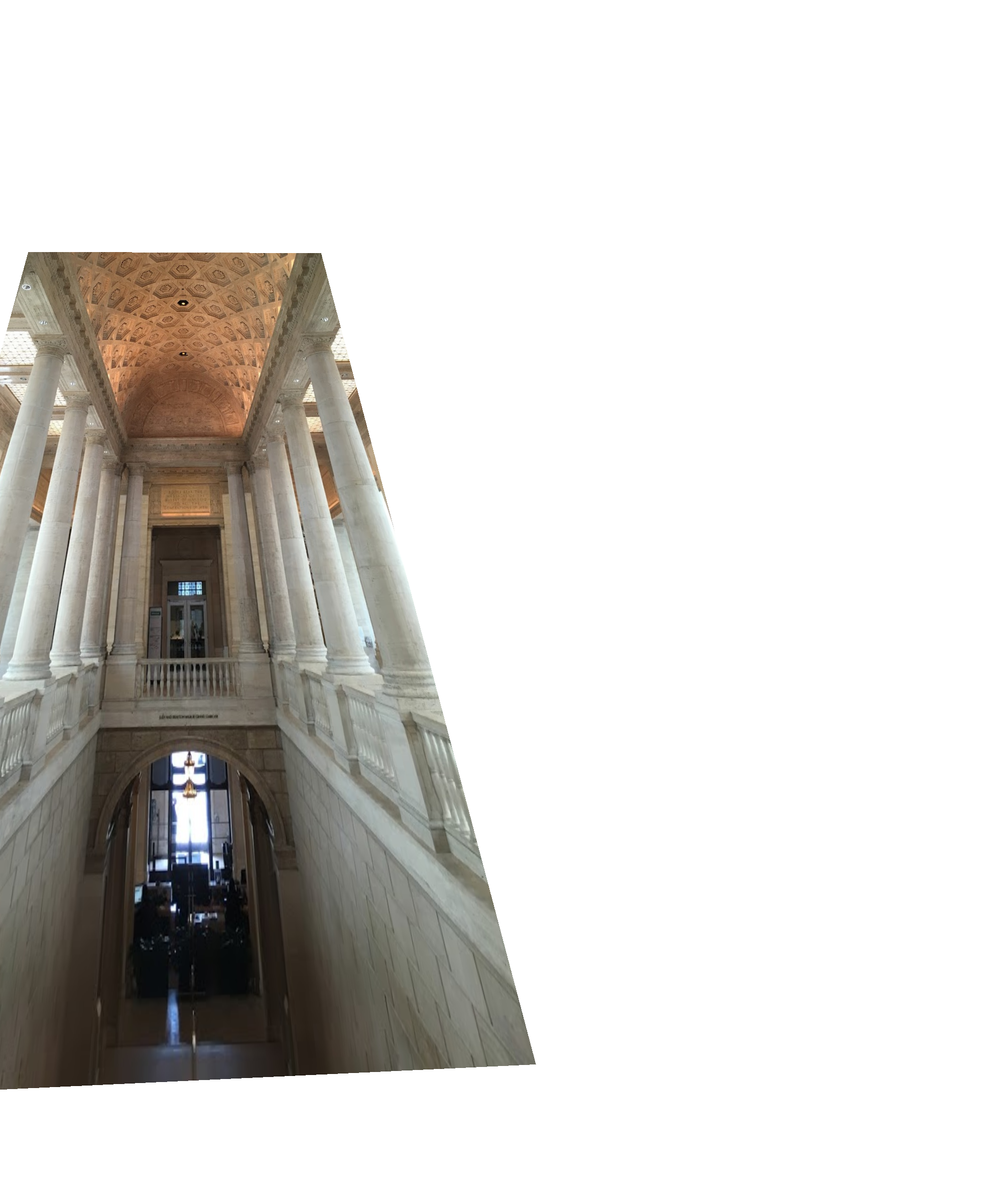
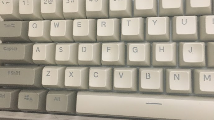
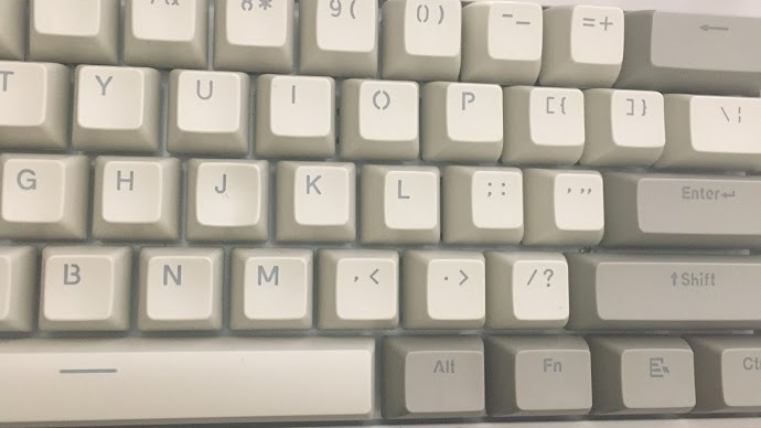
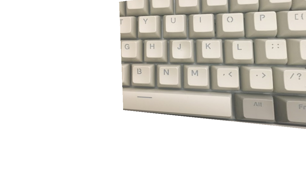
For rectification, I took a picture of something I knew had a planar surface then picked points on it that corresponded to a square. The best results were typically in images where the planar surface was large.

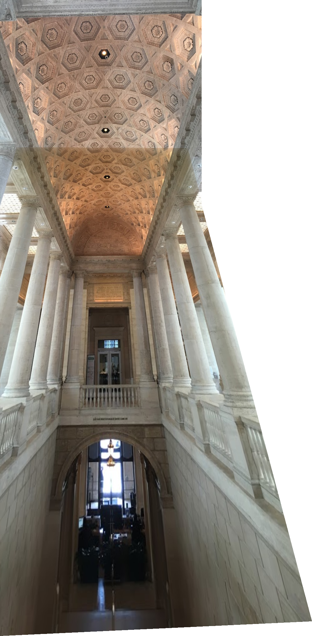
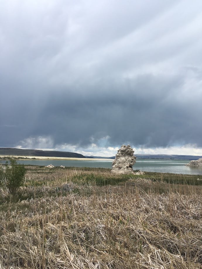
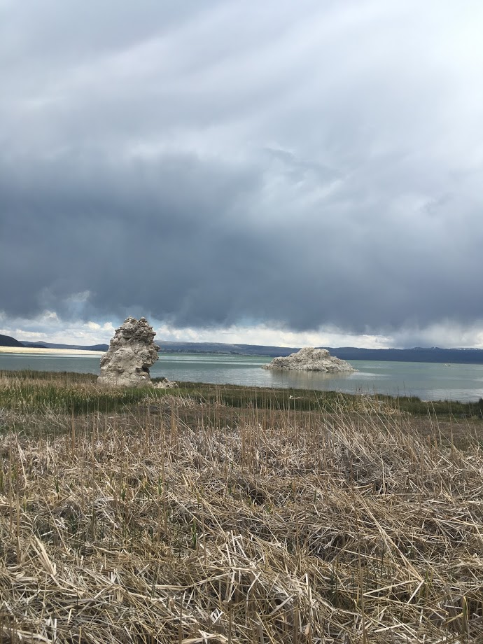
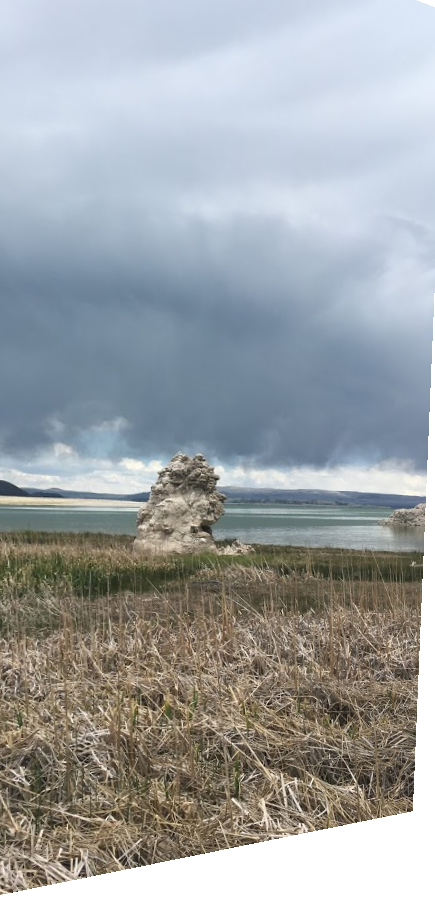
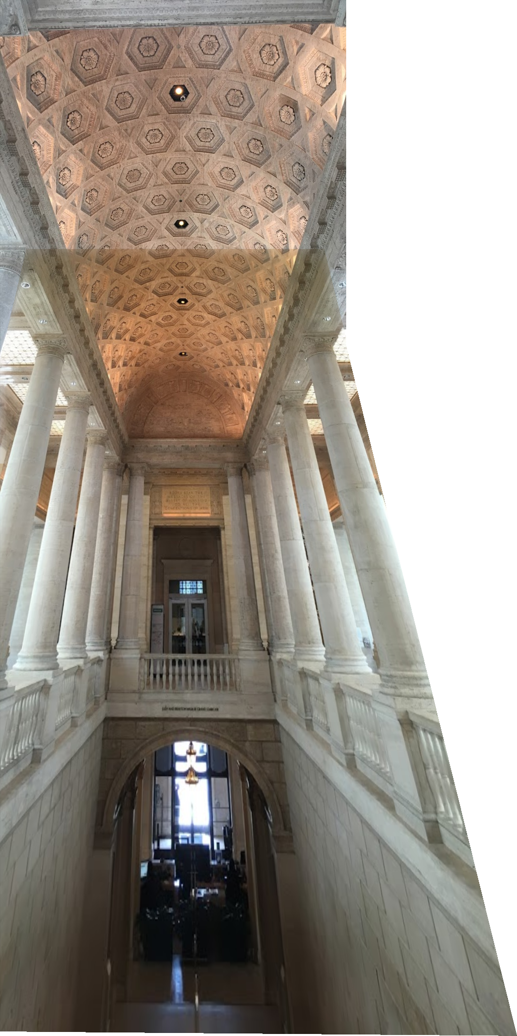
Mosaics:

I had the best luck with leaving one image unwarped and warping others onto its projection. I did this about the same way that I did rectifications, except instead of planes to squares, I used the sets of interest points I had selected to create the homography. I did the same inverse warp with a pixel 'canvas' as I did with rectification. After doing the warp, I padded (if necessary) the warped image and destination image so that they would have the same canvas. I made masks for each of their NaN values so that I could set them equal to the other image to make the sitching look nice. To avoid sharp edge artifacts, I used the stack blender from project 2 to smooth out the seams.

Autostitching

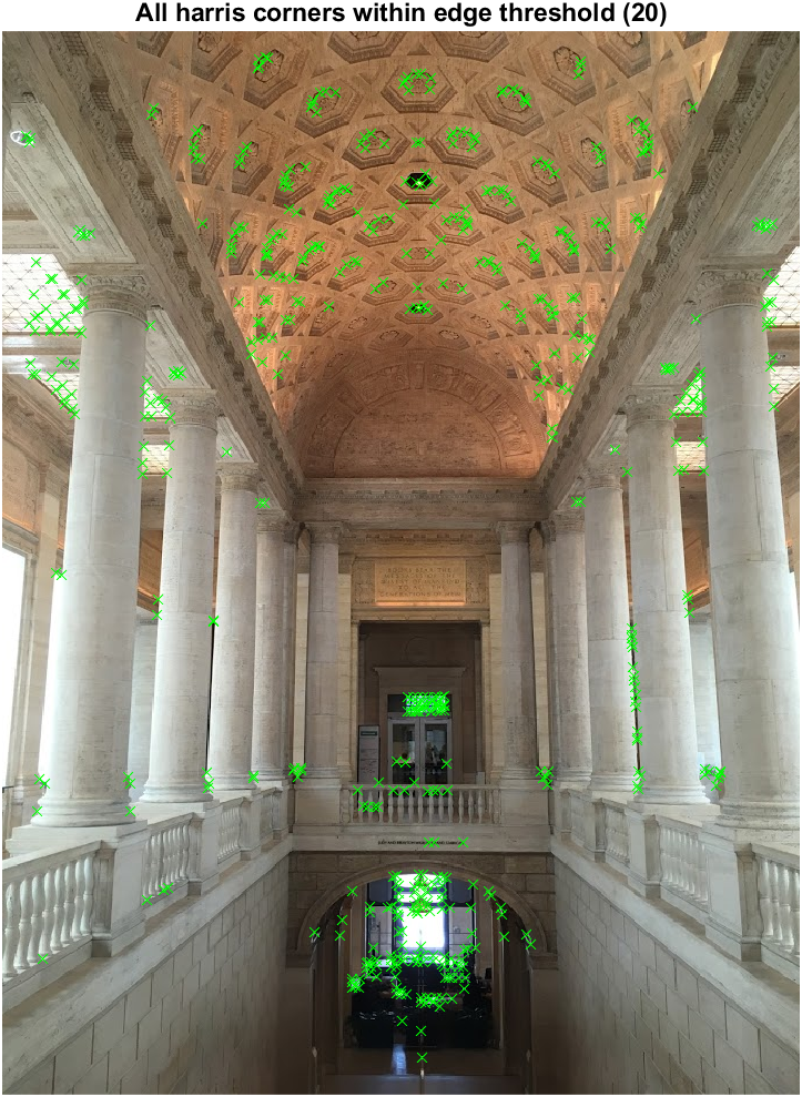
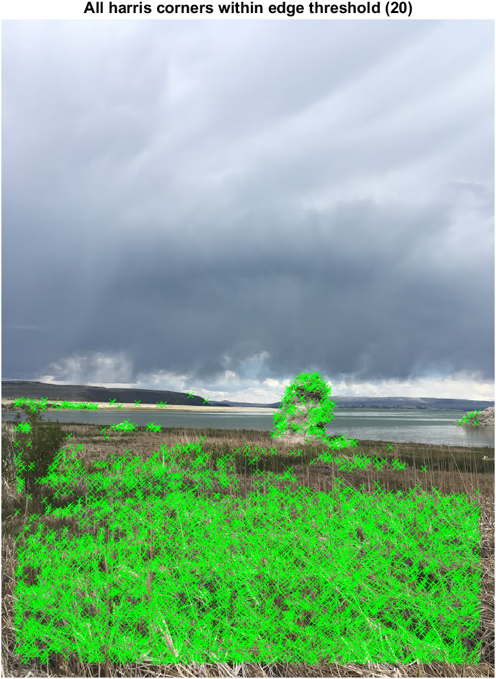
In order to do autostitching, we had to implement the MOPS paper. The first thing to do is get the harris corners, which I did using detectHarrisFeatures.

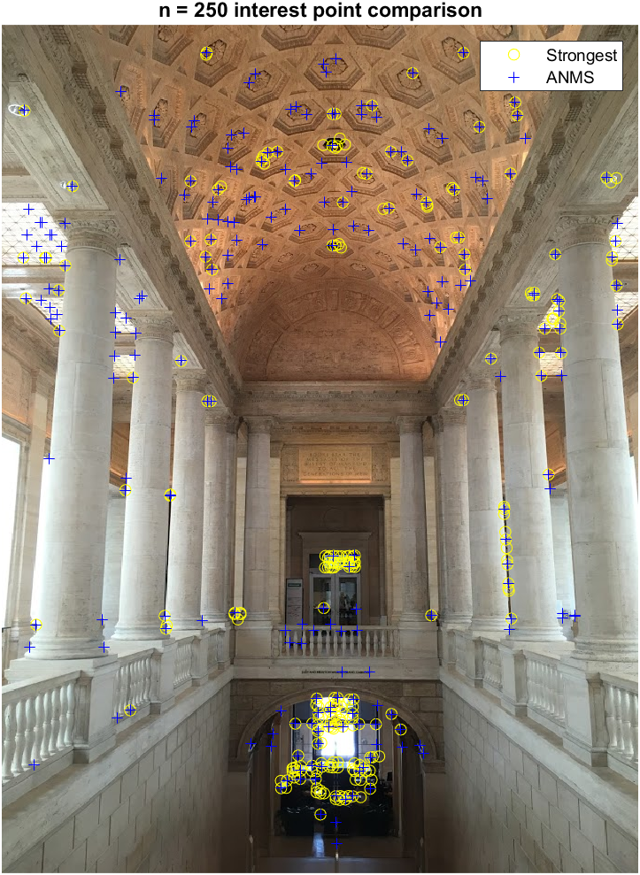
But this is far too many corners to do anything with, so we need to get rid of outliers and bad points. The first thing I implemented was the ANMS algorithm. This is meant to keep only the points that are not only strong, but also spaced far apart as possible. I did this in MATLAB by making an array that acted as a grid of cornerpoints. Each (i,j) pair represented a comparison between points. The elements were filled with the distance from a point in row i distance to points in column j. I could index into this with another array that I made that compared a points metric to another using the same rows vs cols setup. I found the minimum distance r_i for each point i from every other point by taking the min of each row. 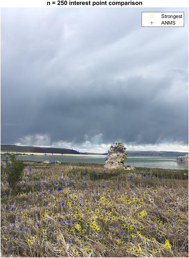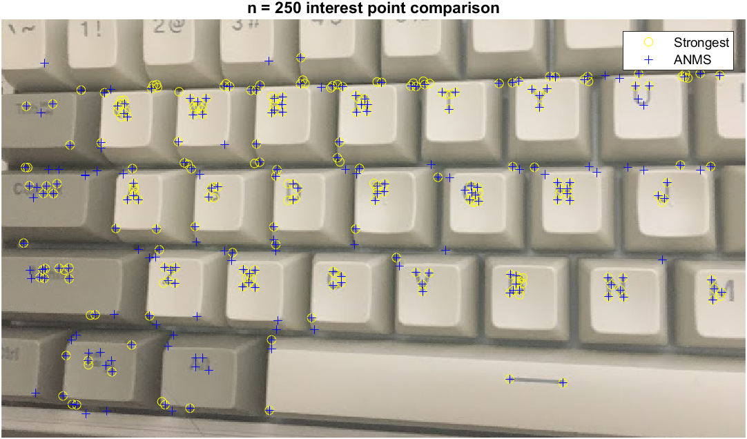Now with these, I used maxk to find the max 500 values in the array of points with their r_is, then finally returned the points that corresponded to the N largest suppression radii.

For comparison's sake, I included the top 500 strongest points as chosen by MATLAB. You can see the points are more spread out when the suppression radius comes into play.

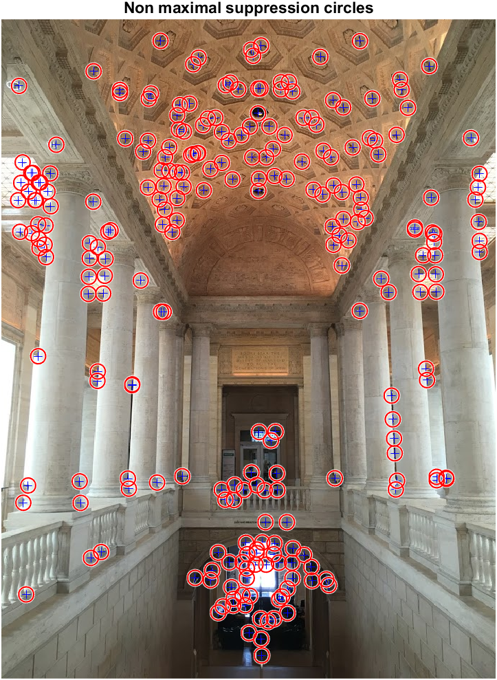
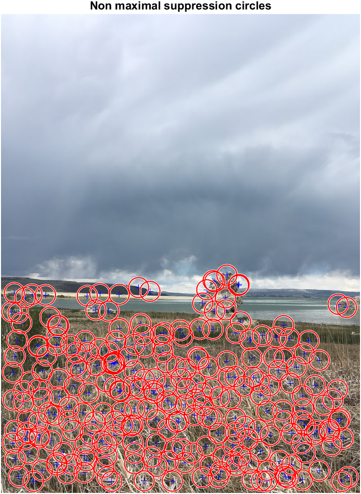
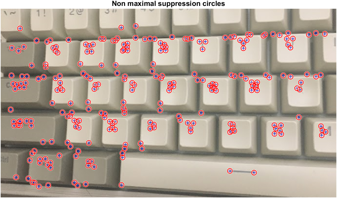
Points with suppression radius:

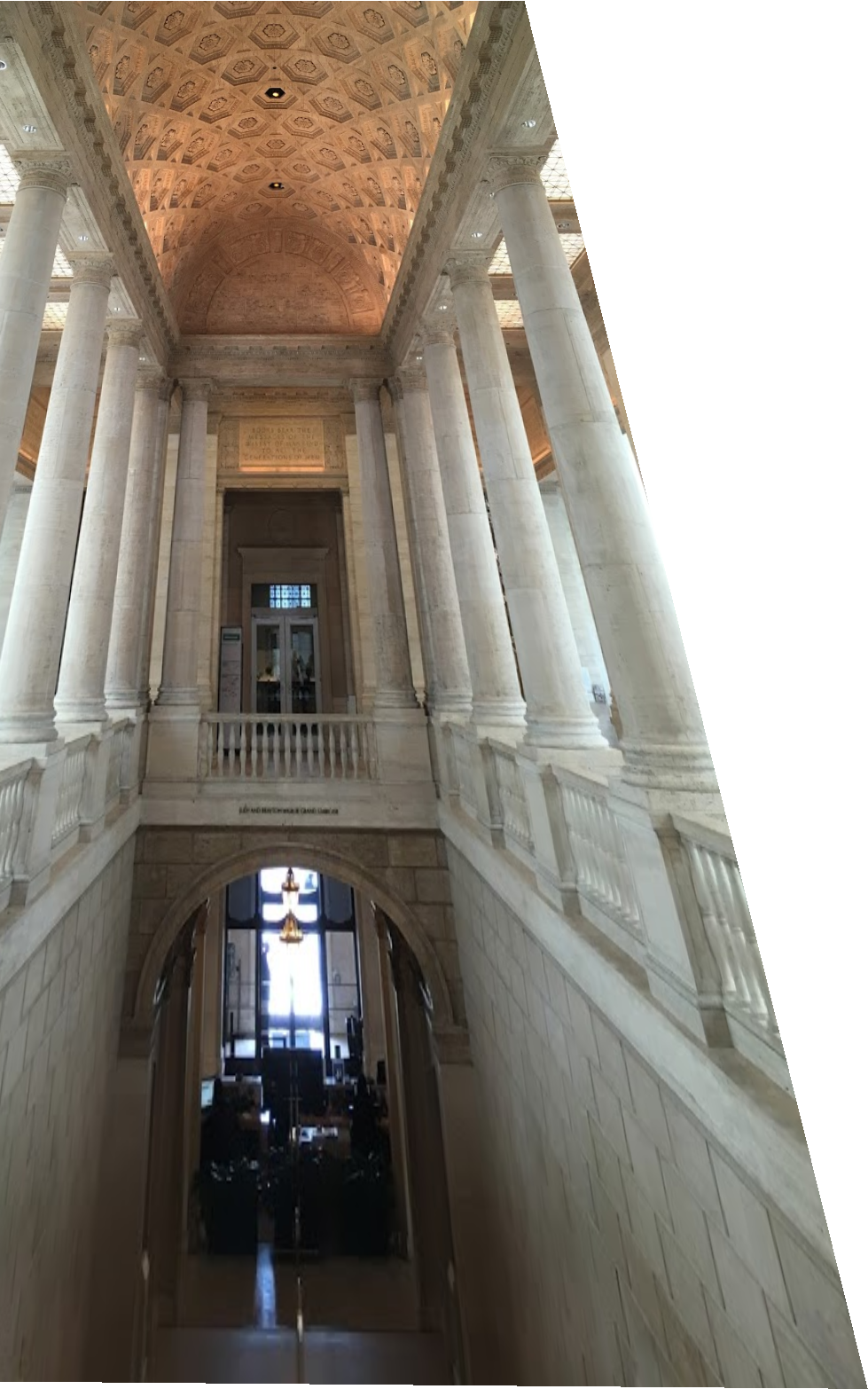
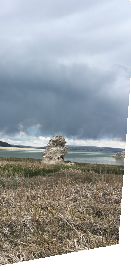
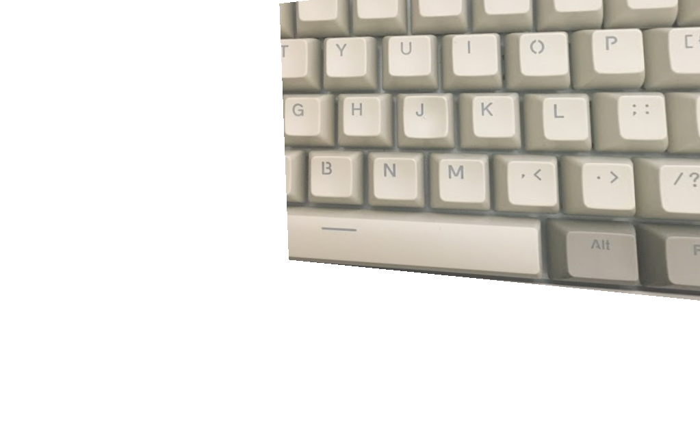
The actual warps:

Auto to manual warp comparisons

What did I learn?

One thing I particularly like about this class, and computer graphics/image processing in general, is the visual debugging element to it. I love being able to tweak a few paramaters and watch how my result changes from something incomprehensible to something that looks pretty good. In the case of this project, I got the opportunity to that with homographies. At the start of this project, I didn't get what it meant to do a prospective transformation and had sort of a hard time imagining what it meant to warp an image with no depth, but now I can see that it's more like if I had two pictures on film, and I was trying to orient them in such a way that it made an overlap to look like a new image in 2D from my head on perspective.

Also-- the paper was fun to read and implement!