This project is an extension of the previous part of the Image Warping and Mosaicing project. Before, we had to manually define point correspondences between a set of pictures to create a mosaic of the images. This time, we want to create a system that will automatically find these correspondences and stitch them together to create the resulting panorama. Many of the parts in this project are inspired by this research paper by Brown et al.
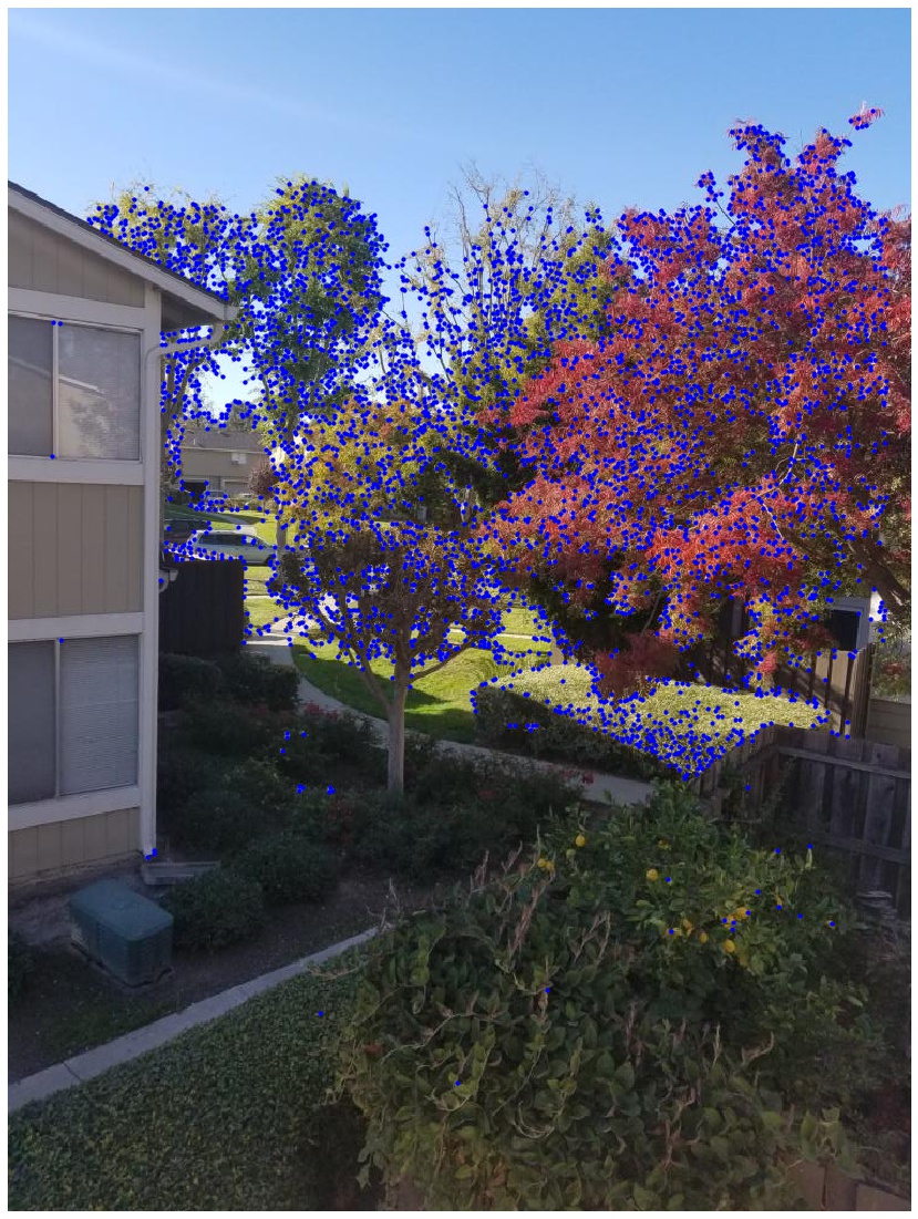
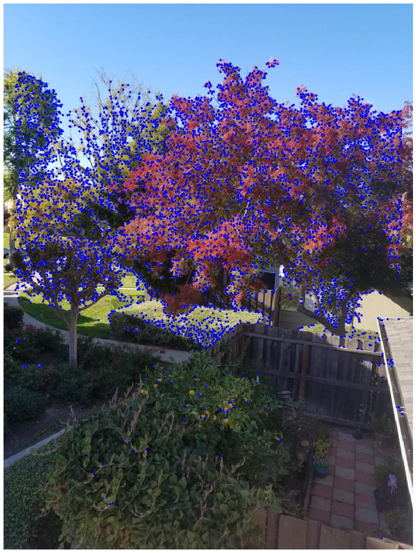
When choosing point correspondences between images, we want to choose good features that are prominent and easy to localize. Good features that satisfy these properties are corners. Because detecting corners in images from scratch is a daunting task, we will use a Harris Interest Point Detector to find these corners in our images automatically. The results of the detector on sample images from part A are shown below.
As you can see, the number of detected corner points in the images can range up to the thousands. To reduce the number of interest points we have to consider, we will use Adaptive Non-Maximal Suppression (ANMS). In ANMS, we want to have evenly distributed points in the image but also have a fixed number of interest points. This can be done by calculating the minimum suppression radius r for each point and keeping a set amount of points with the largest radius. f is the corner strength function provided by the Harris detector.

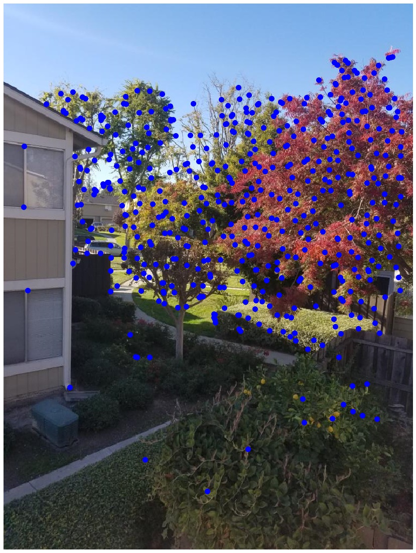
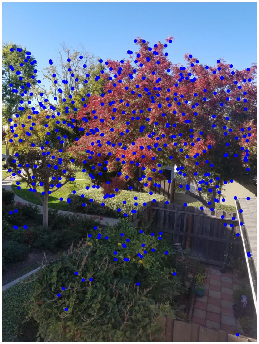
After implementing this technique, the number of features we have to consider is significantly reduced:
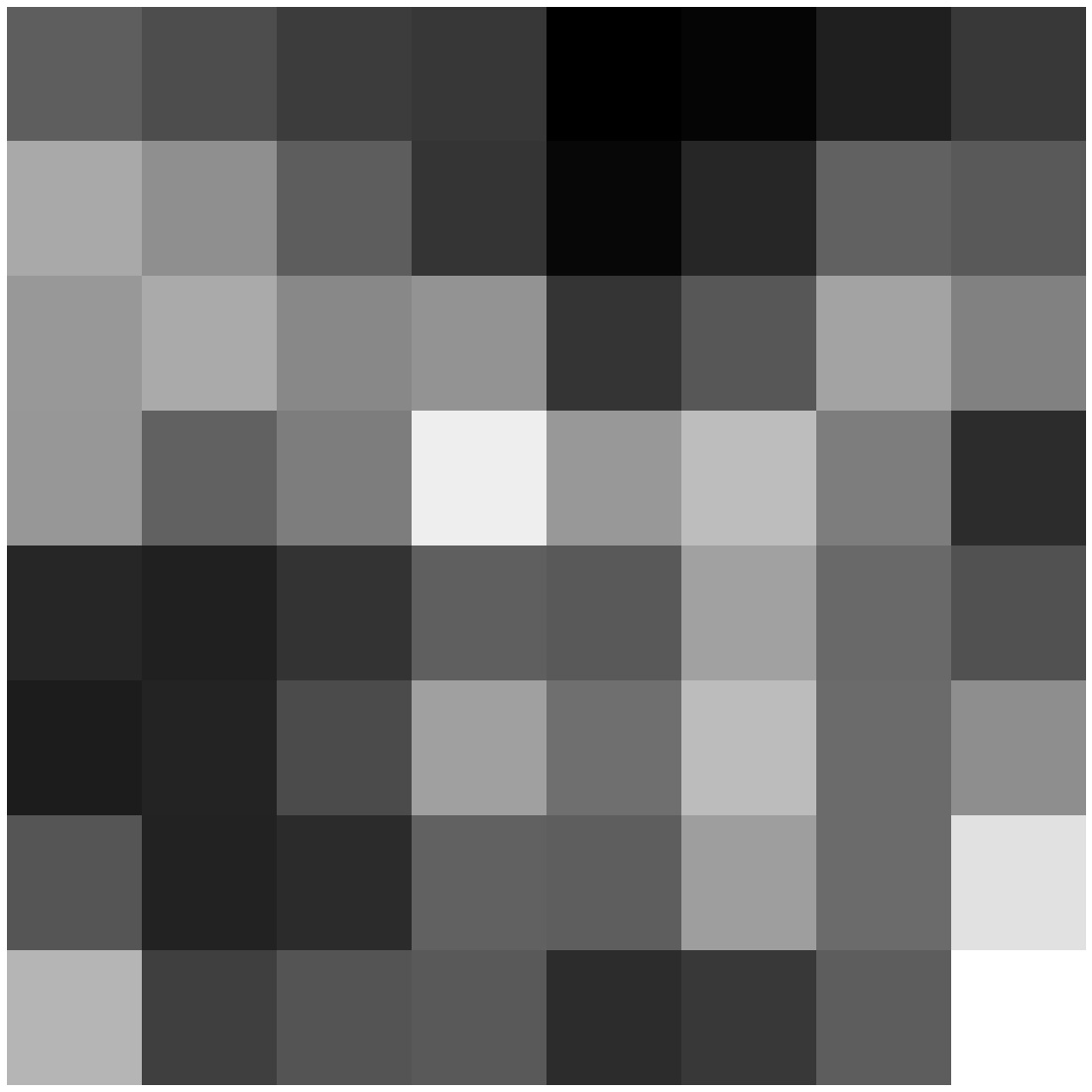
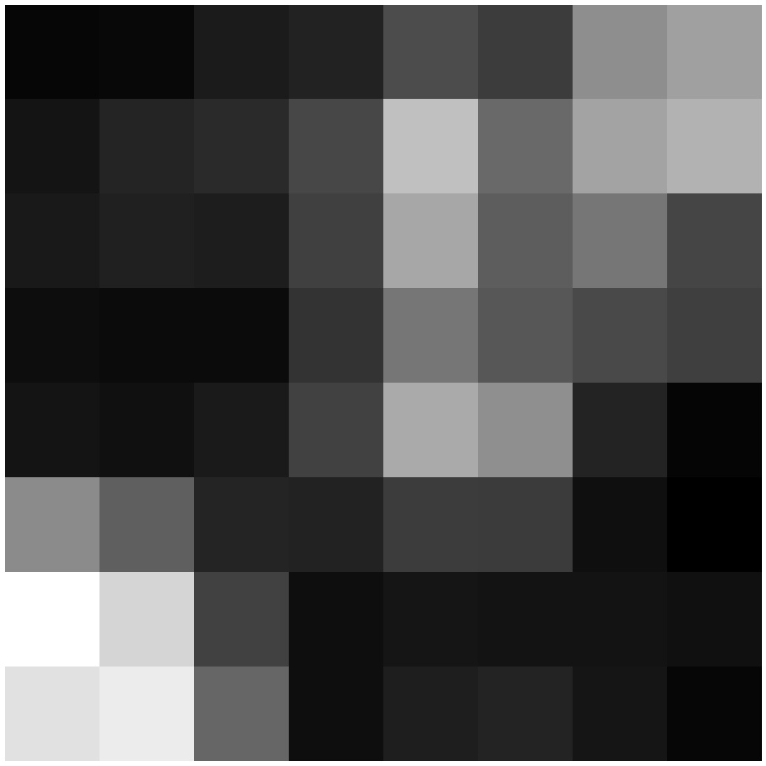
Now that we have a selection of interest points in our images, a question that arises is how can we match points in one image to points in another image? The answer is feature descriptors. For each interest point in our images, we will sample a 40x40 square around the point, downsample it into an 8x8 patch with a Gaussian filter, and finally, normalize it such that the pixel values of the patch have a mean of 0 and a standard deviation of 1. Some example features are shown below.


We can now start matching points together. For each 8x8 feature in the first image, I will compare it to every 8x8 patch in the second image and use the sum of squared differences to find a pair of patches that is the best match. To reject outliers in our matches, we will also determine the pair of patches that is the second-best match and keep the best pair where the ratio between the best pair and the second-best pair is lower than a certain threshold. This step is necessary to keep the patches that are significantly better than the rest of the compared features. After implementing this step, our result is as follows:

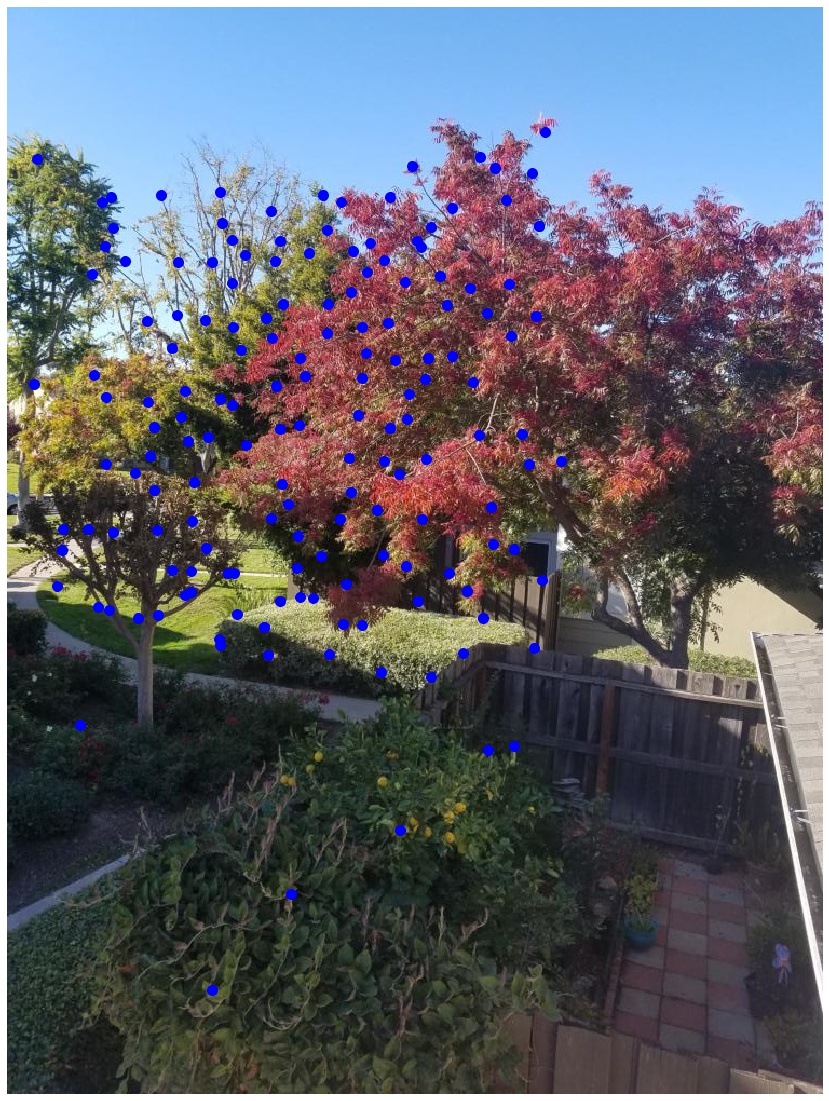
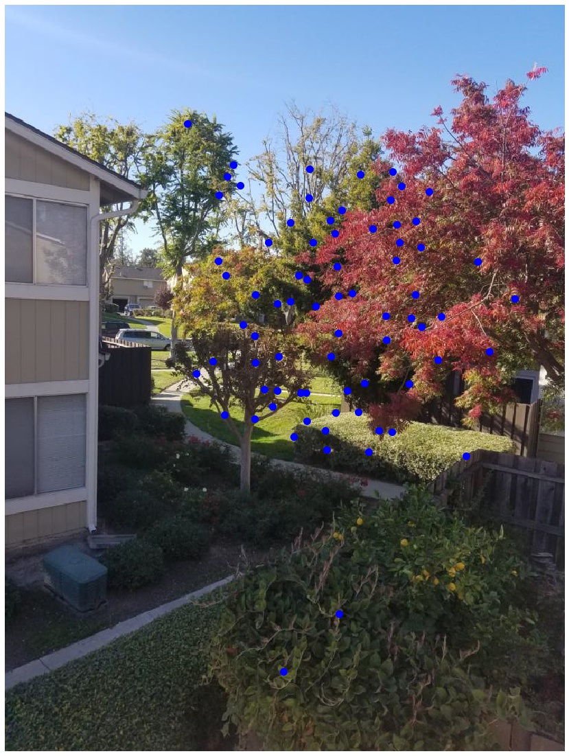
To robustly remove bad matches in our current set of correspondences, we will use random sample consensus. In this technique, we will randomly sample 4 different point correspondences from our images, compute the homography transformation between them, calculate how many point correspondences satisfy the homography transformation below a certain threshold, and finally keep the largest set of satisfied points. Our sample images have had their point correspondences reduced from a few thousand points to only 75 points.
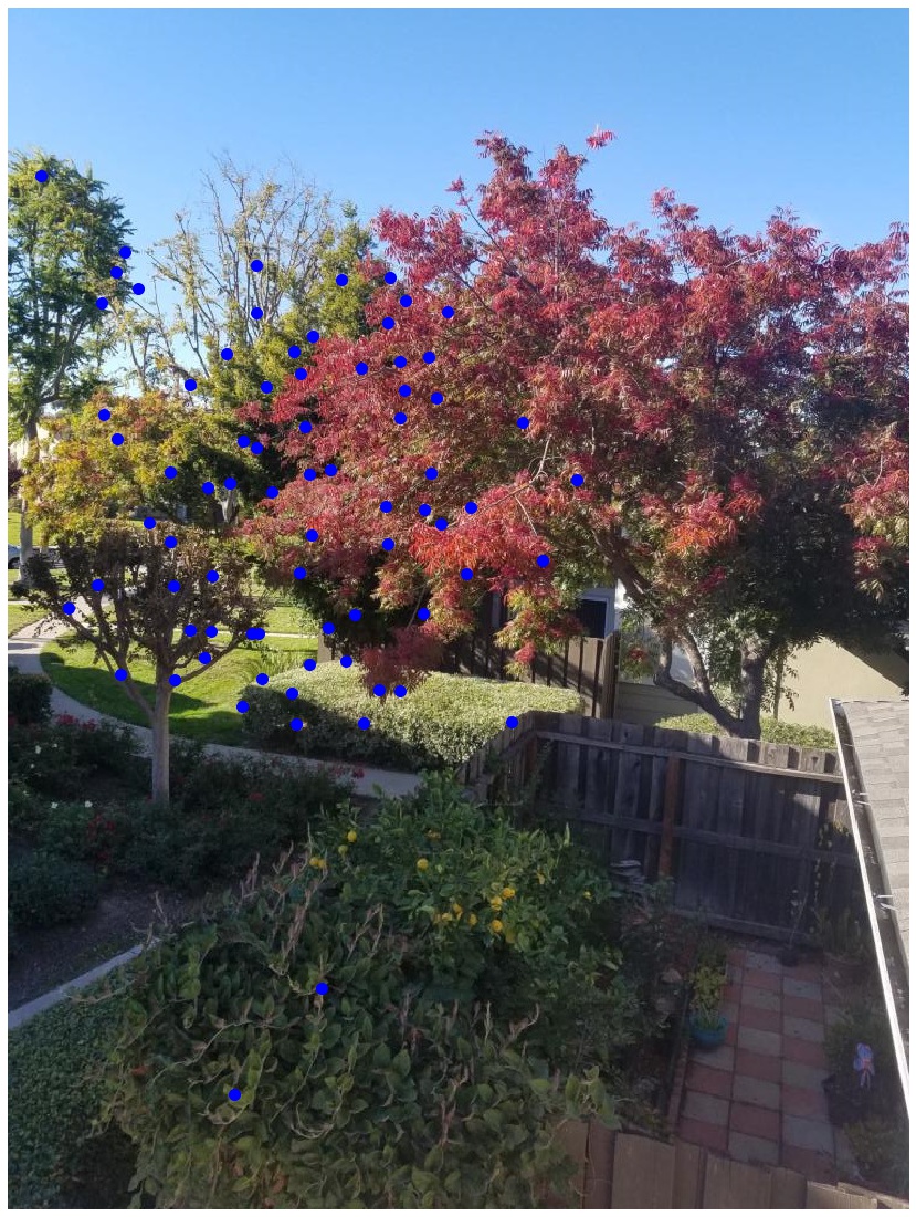
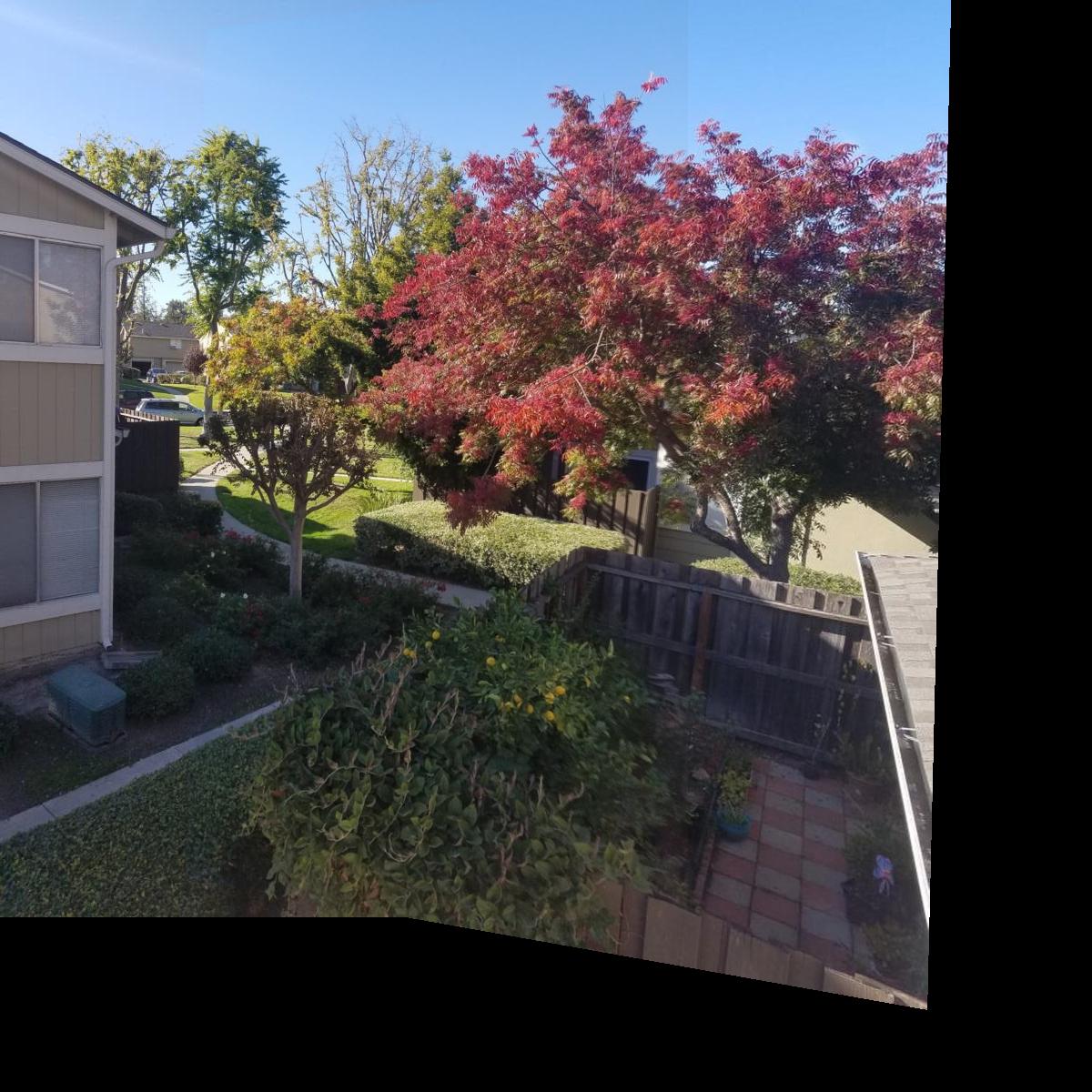
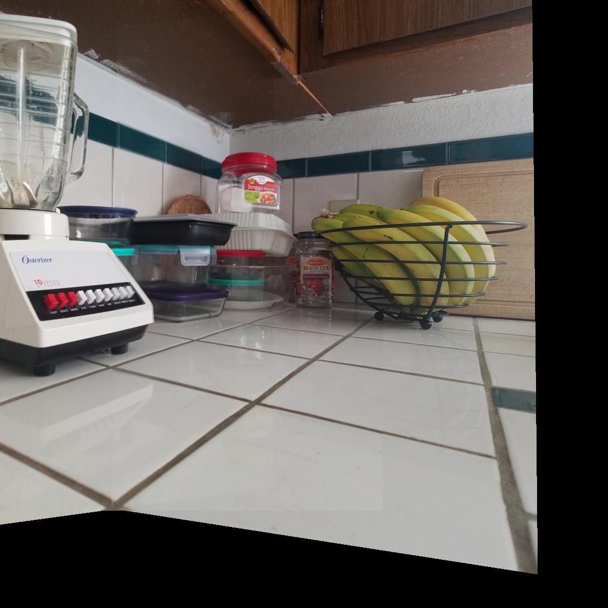
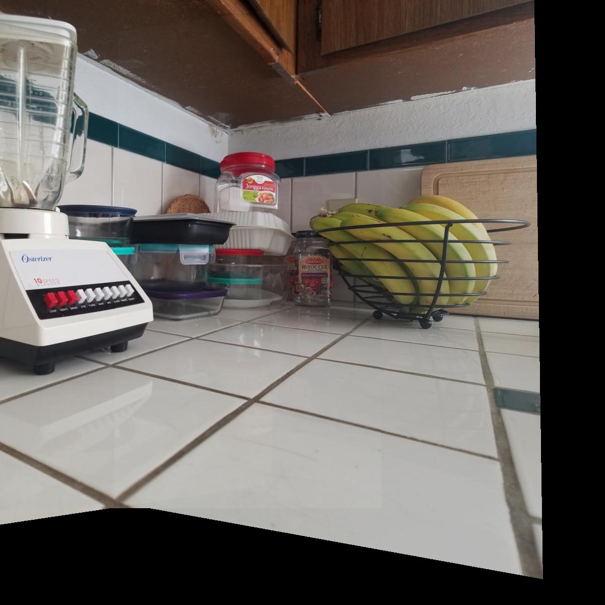
We have finally produced our best set of point correspondences. It is now time to start blending the images together to create mosaics. I will reuse the same blending algorithm that was implemented in part A to produce the panoramas. I will also compare side-by-side the manually defined correspondence mosaics from part A against the automatically produced ones.

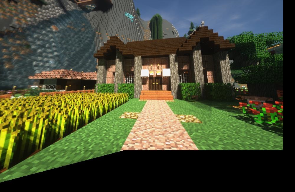
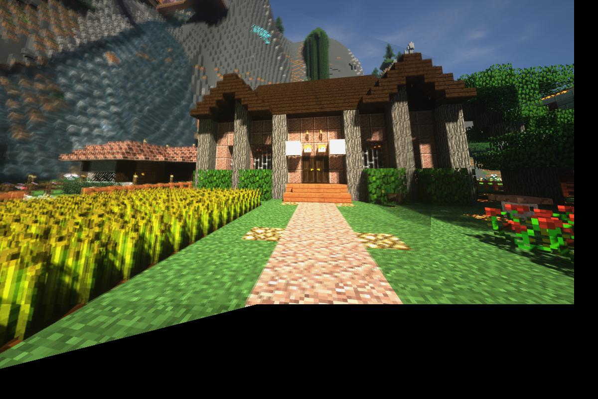
Let's also see how well the algorithm does on a set of new images. Below are the mosaics of a few images I took while playing Minecraft. As shown in the automatic mosaic, the bottom-left side of the image appears to be more blurry compared to the manual mosaic. This is due to the detector not being able to find a robust point correspondence in that area of the image compared to the other parts of the pictures.
Overall, this project was very insightful to me for understanding the mathematics behind image rectification and mosaic creation. The coolest thing that I learned is that not all detection problems in the field of computer vision require machine learning models to solve them. Sometimes linear algebra is all you need to accomplish your goals!