Overview

In this project, I learned how to compute the homography matrix to apply projective transforms to images and produce cool images.

Part 1: Image Warping and Mosaicing

Shooting Pictures

The first part of the project involved shooting the pictures I would be working with. I shot all of the images (other than the last one) using my phone. I made sure for the images I'd be using for forming mosaics that there'd be enough overlap to have a solid homography computation.

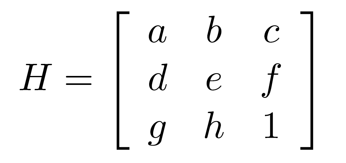
Recover Homographies

The homography matrix is a 3x3 matrix of the following form. We need at a minimum 4 correspondence pairs between the source and destination images to find the homography matrix because it has 8 degrees of freedom.

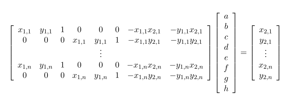
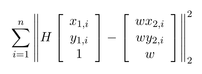
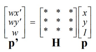
Once I computed the least squares solution to the above linear system of equations, I reshaped the vector back into a matrix H. We can find the transformed pixels by computing p' as below, then dividing the first 2 elements by w.

Warping and Image Rectification

Now that we've computed the homography matrix, we can use it to transform and warp images to one another. I utilize the inverse of the homography matrix to perform inverse warping, which constructs the transformed image using pixels of the original image.

Image rectification involves finding points in the original image around some object, finding the homography matrix that warps the points into a parallel shape, like a rectangle, and using the inverse homography matrix to transform the original image so that the object appears frontal parallel.

Blending Images into Mosaics

Using our perspective warping functionality, we can do other cool stuff like form mosaics. To do so, we warp one image using a homography computed from certain key matching features. Defining more correspondences improves the accuracy of the homography, and otherwise, I defined the correspondences manually based on how well the features matched. After warping the first image to the second, I blended the images together to form a mosaic. I tried different blending methods such as linear blending, max blending, pyramid blending, but I found that max blending worked best for my images.

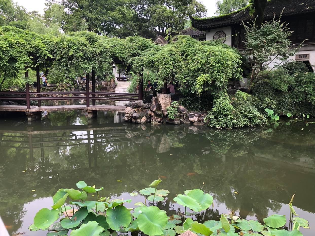
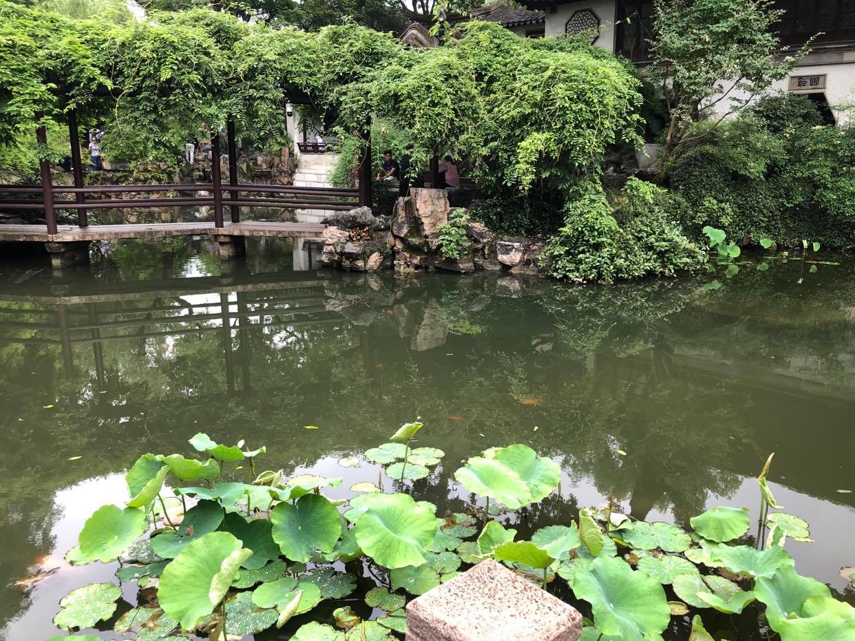
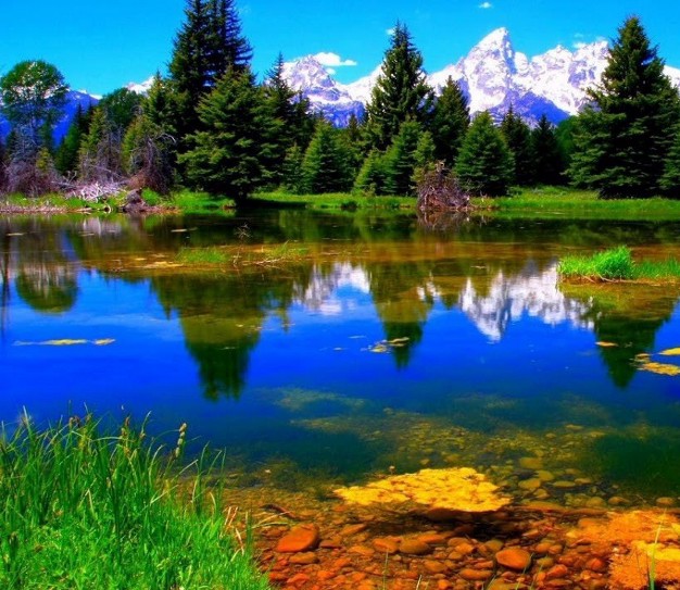
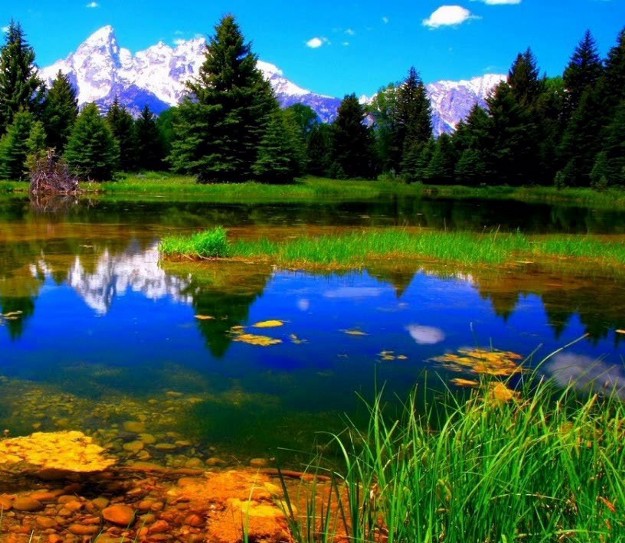
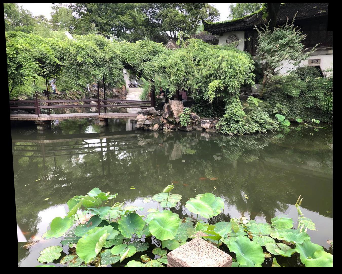
Pond

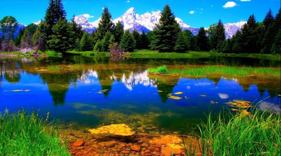
Nature

Learnings

The most coolest part of this section of the project was rectifying images. I found it fascinating that image warping was able to recover such a detailed representation of objects in parallel form, despite not being given much details initially that we can see from our own eyes. A lot of detail does exist in the initial image that our eyes do not notice, but the machine can.

Part 2: Feature Matching For Autostitching

For this part of the project, we follow the techniques in this paper to automatically identify matching features between images, which we can then use to stitch the images together with the techniques used in the first part of the project. The process the paper describes is as follows:

1. Harris Interest Point Detection
2. Adaptive Non-Maximal Suppression (ANMS)
3. Feature Descriptor Extraction
4. Feature Matching
5. Random Sample Consensus (RANSAC)
6. Warp and Blend

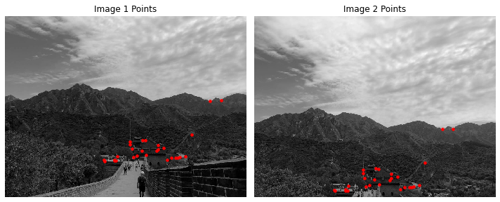
Harris Interest Point Detection

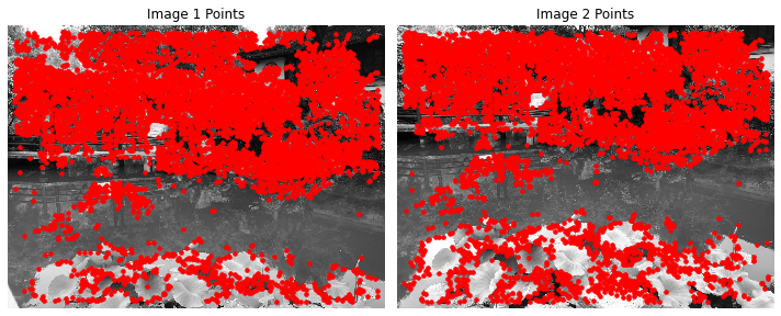
Let's start with Harris Point Detection. The Harris Point Detector operates by detecting corners in an image locally, computing a "corner strength" value for each pixel in the image. Notice that our points are very dense in certain areas, which brings us to the next step.

ANMS

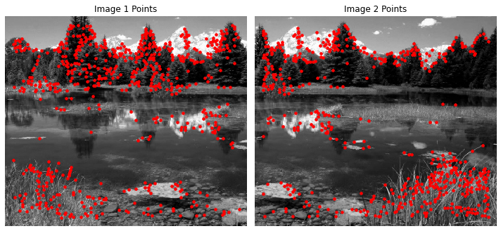
ANMS ensures that our points are well distributed throughout the image and not densely packed. It goes through all of the points that our harris detector found, and their minimum supression radius. It then sorts our feature points according to the highest radius values and retains the top 500 points.

Feature Descriptor Extraction

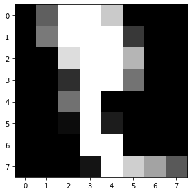
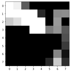
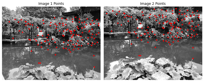
Our next step involves extracting axis aligned feature patches centered about our feature points. The feature patches are generated by finding a larger 40x40 window, applying a gaussian filter to smoothen it, and subsampling to a 8x8 patch. Here are some example patches from our pond image:

Feature Matching

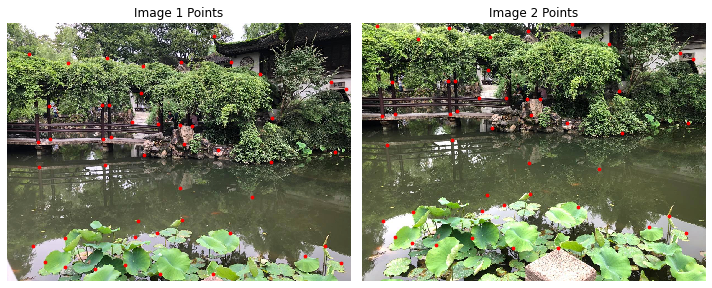
Using these 8x8 patches for each point, we can perform feature matching. We do so by iterating through all the patches in the first image and computing its ssd with all the patches in the other image to find nearest neighbors. We then use the first 2 nearest neighbors to compute a ratio E_NN1 / E_NN2, which we used to filter points if the ratio was over a certain threshold. I found that the threshold .4 worked for most of the images. Using the ratio ensured that our points were a decent match for each other and that all the other points did not match as well, thus reducing the risk of mismatches.

RANSAC

Our last step was using RANSAC to eliminate outlier points because outliers make homography calculation awful. RANSAC follows the following steps:

1. Select 4 random pairs of points
2. Estimate homography matrix H
3. Find inlier points where SSD(p', H(p)) <= epsilon
4. Keep track of largest set of inliers
5. Repeat 1-4 for X iterations

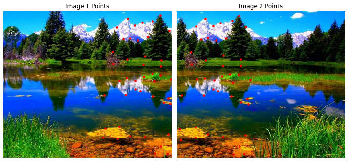
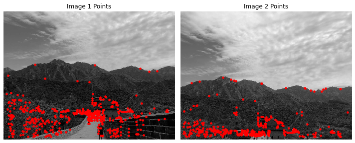
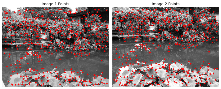
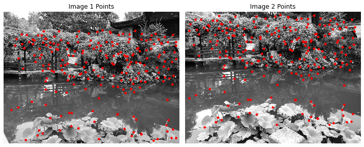
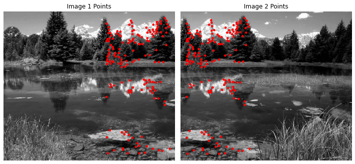
I repeated the steps for 5000 iterations with epsilon=1 and got the following pairs of inliers:

Warp and Blend

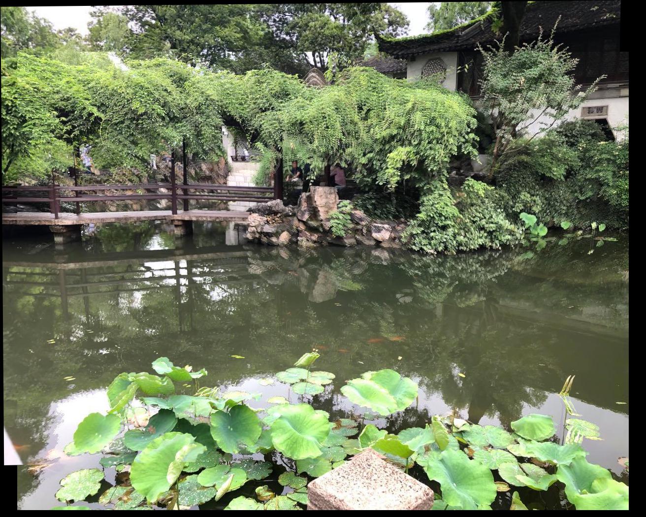
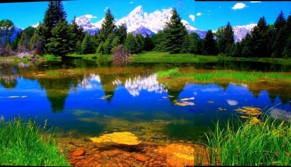
Once we've completed RANSAC and found our largest set of inliers, we use the inliers as correspondence points and follow the same steps as we did in part 1 to generate some stitched images. We compare the results below to the manually generated mosaics on the left. You can see that the automatically computed correspondences result in very similar mosaics or ever better mosaics than the manually selected points.

Pond

Our autostitching approach worked almost the same as our manual method. Somethings like the clovers and fences do appear to be better aligned in the manual approach. There was a somewhat noticable difference in the warp made as seen by the blending artifacts on the bottom left.

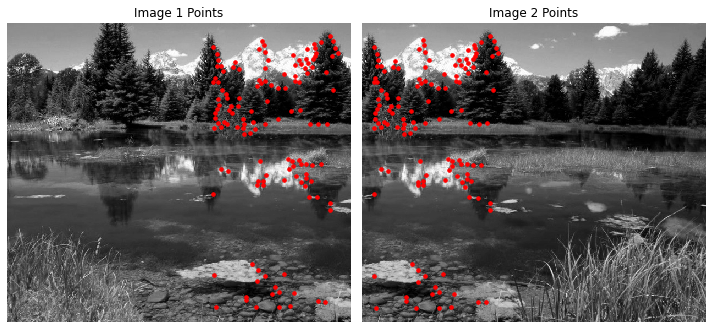
Nature

There were significant improvements with using autostitching for this image. There are no longer and stitching artifacts like there were for the manual mosaic close to the middle.

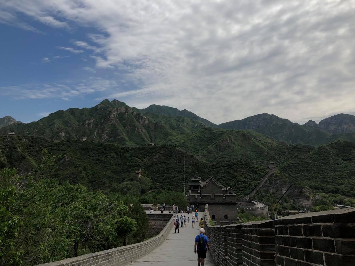
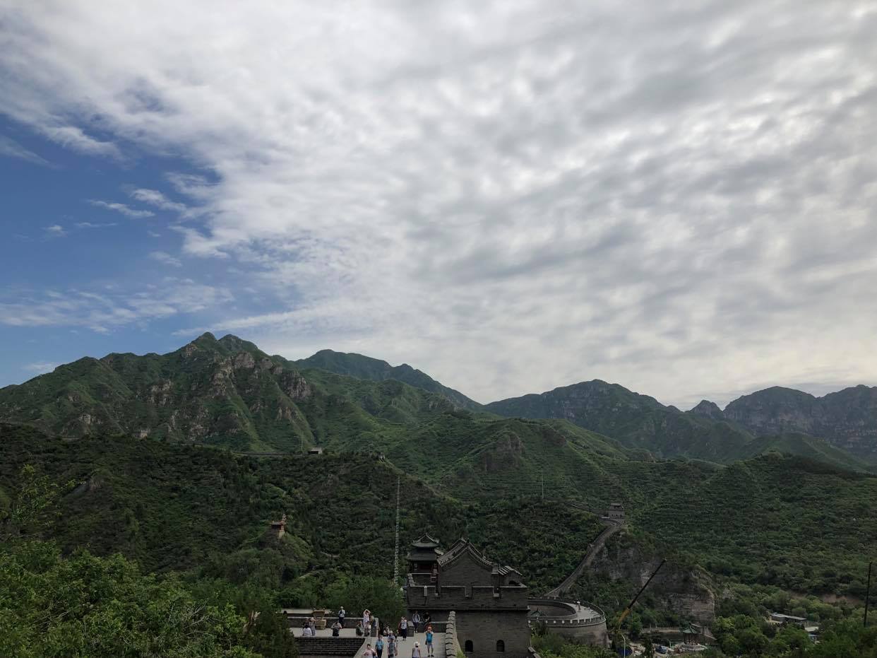
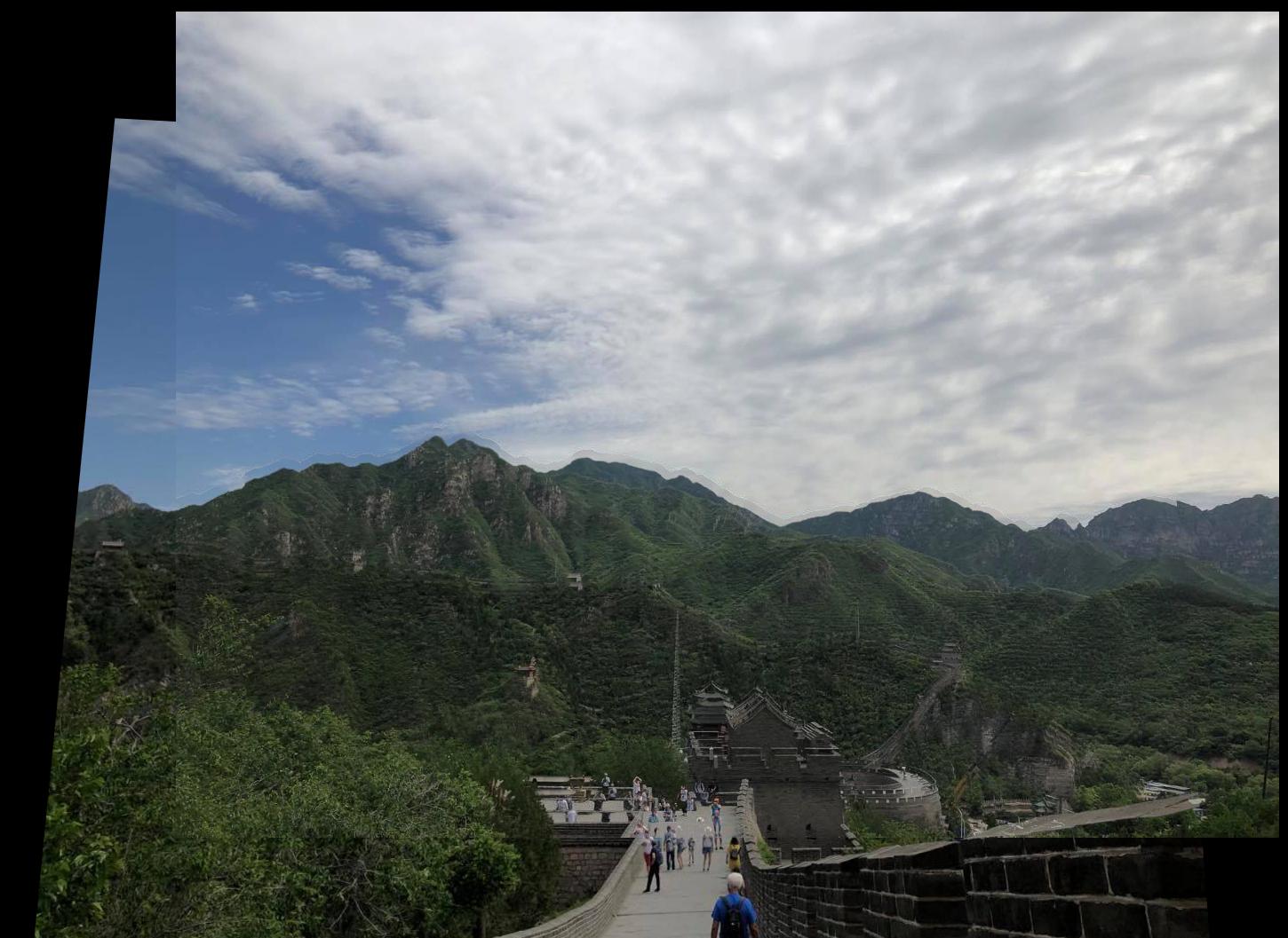
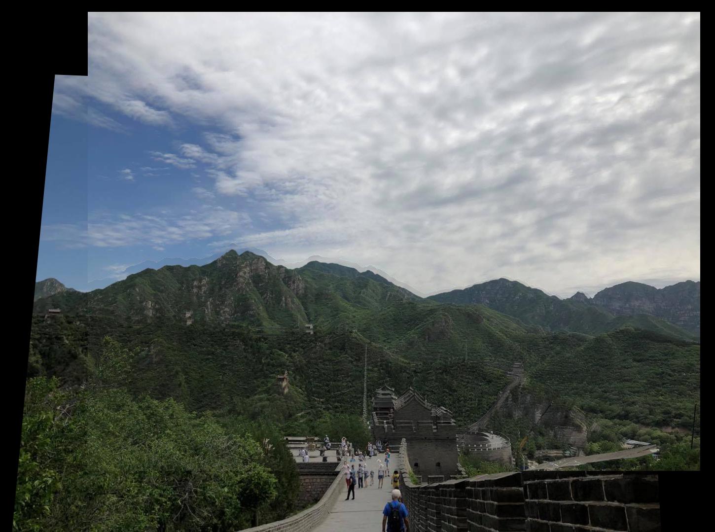
Great Wall

For this image, the warp appeared to be almost exactly the same for both approaches.

Learnings

I really enjoyed the second part of this project as it required me to implement techniques from a research paper. The coolest thing I learned in this part would probably be the feature matching technique used with feature patches and nearest neighbors. I just thought it was interesting how feature matching was done completely mathematically, without any special techniques with heuristics.