Image Warping and Mosaicing
Table of Contents
1 Introduction
In this project, I implemented image mosaicing. I combined two images and create an image mosaic by
registering, projective warping, resampling, and composing them.
2 Image Warping and Mosaicing
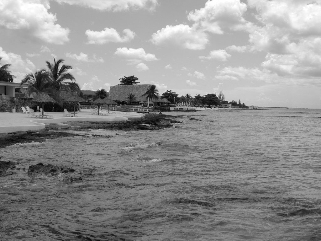
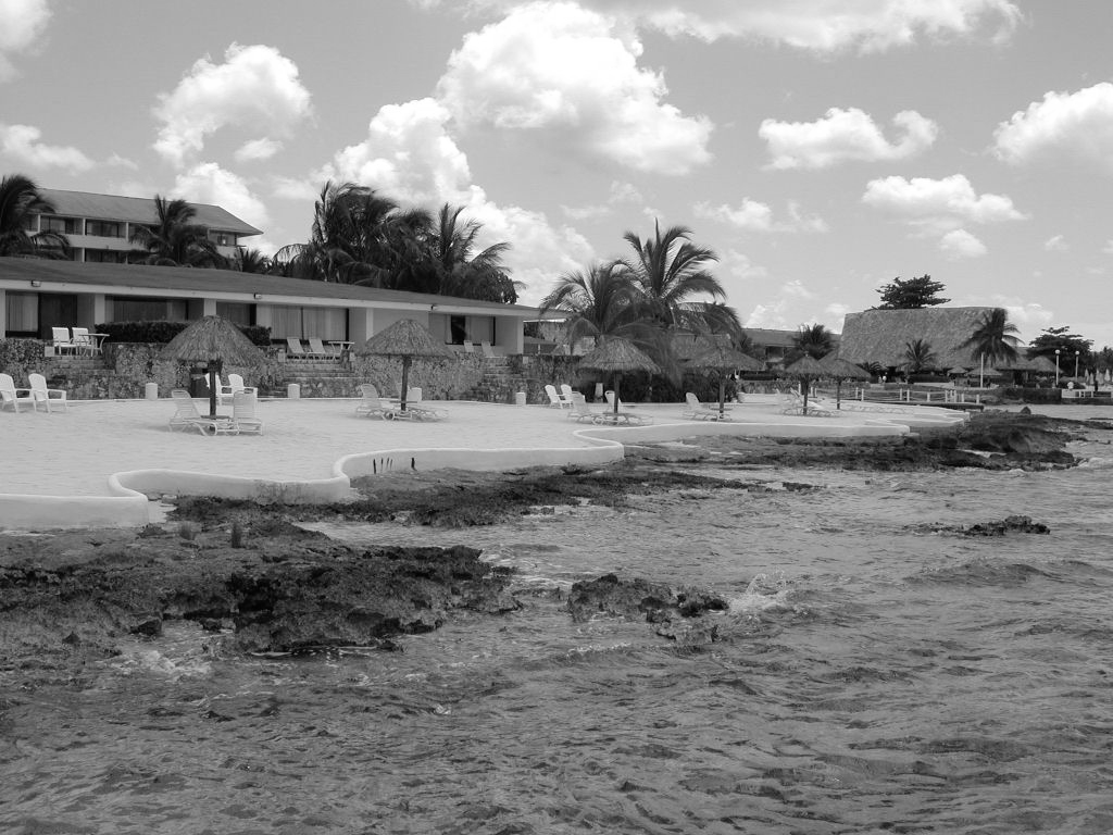
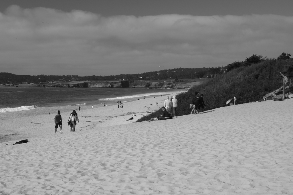
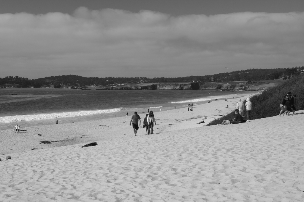
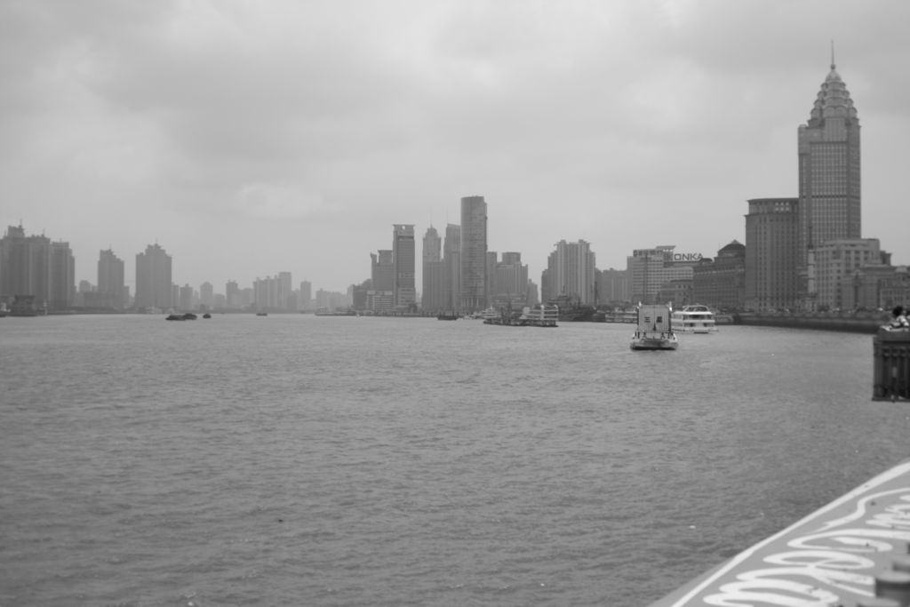
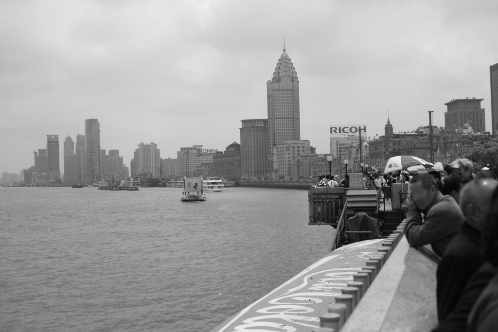
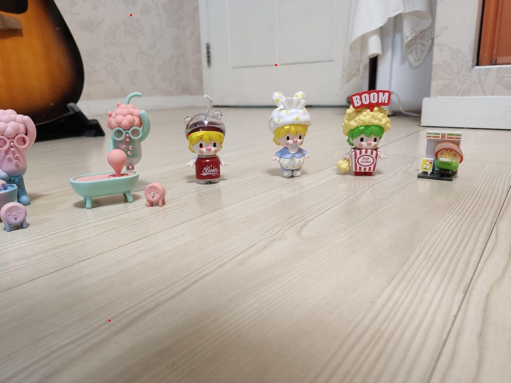
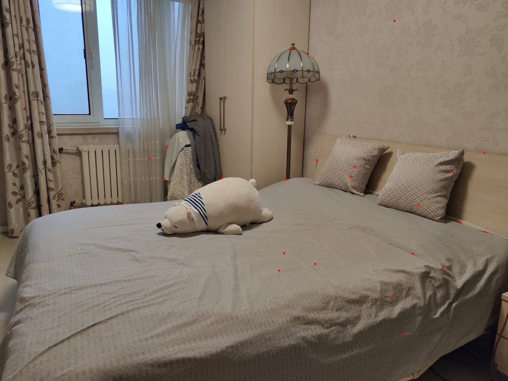
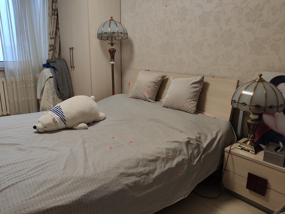
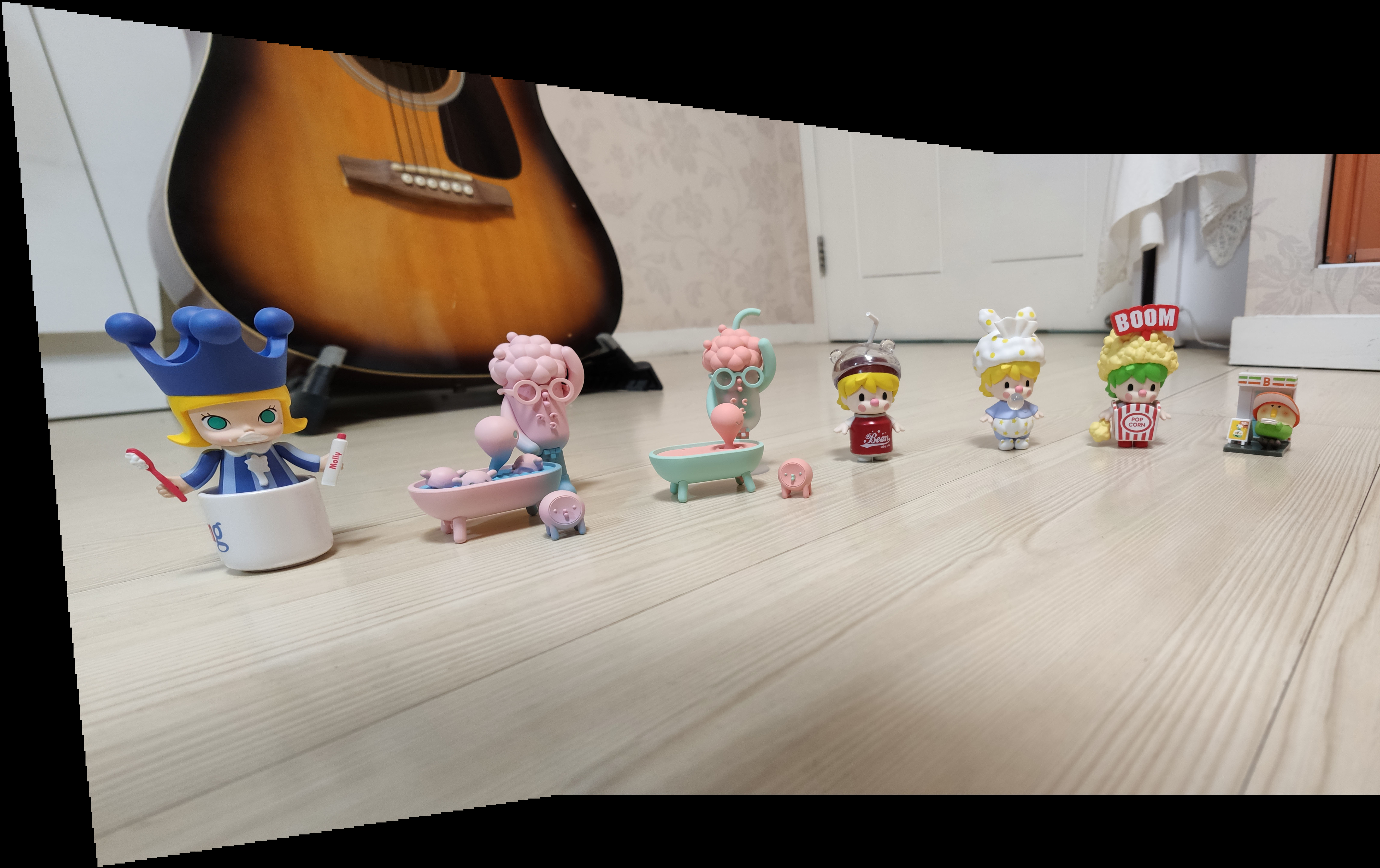
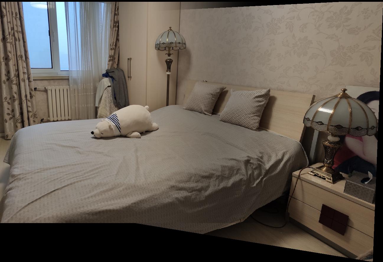
2.1 Shoot the Pictures


2.2 Recover Homographies
Before warping the images into alignment, I need to recover the parameters of the transformation between each pair of images.
The transformation is a homography: p’=Hp, where H is a 3x3 matrix with 8 degrees of freedom.
One way to recover the homography is via a set of (p’,p) pairs of corresponding points taken from the two images.
My homography functions takes the image1 points and image2 points as arguments. They are n-by-2 matrices holding the (x,y) locations of n point correspondences from the two images and H is the recovered 3x3 homography matrix.
To solve homography in python, I used numpy.lstsq, which approximates the overdetermined system using the least square method.
2.3 Warp the Images
After discovering the homographies, we need to apply the transformation matrix \(H\) to all the pixels. I used forward wrapping.
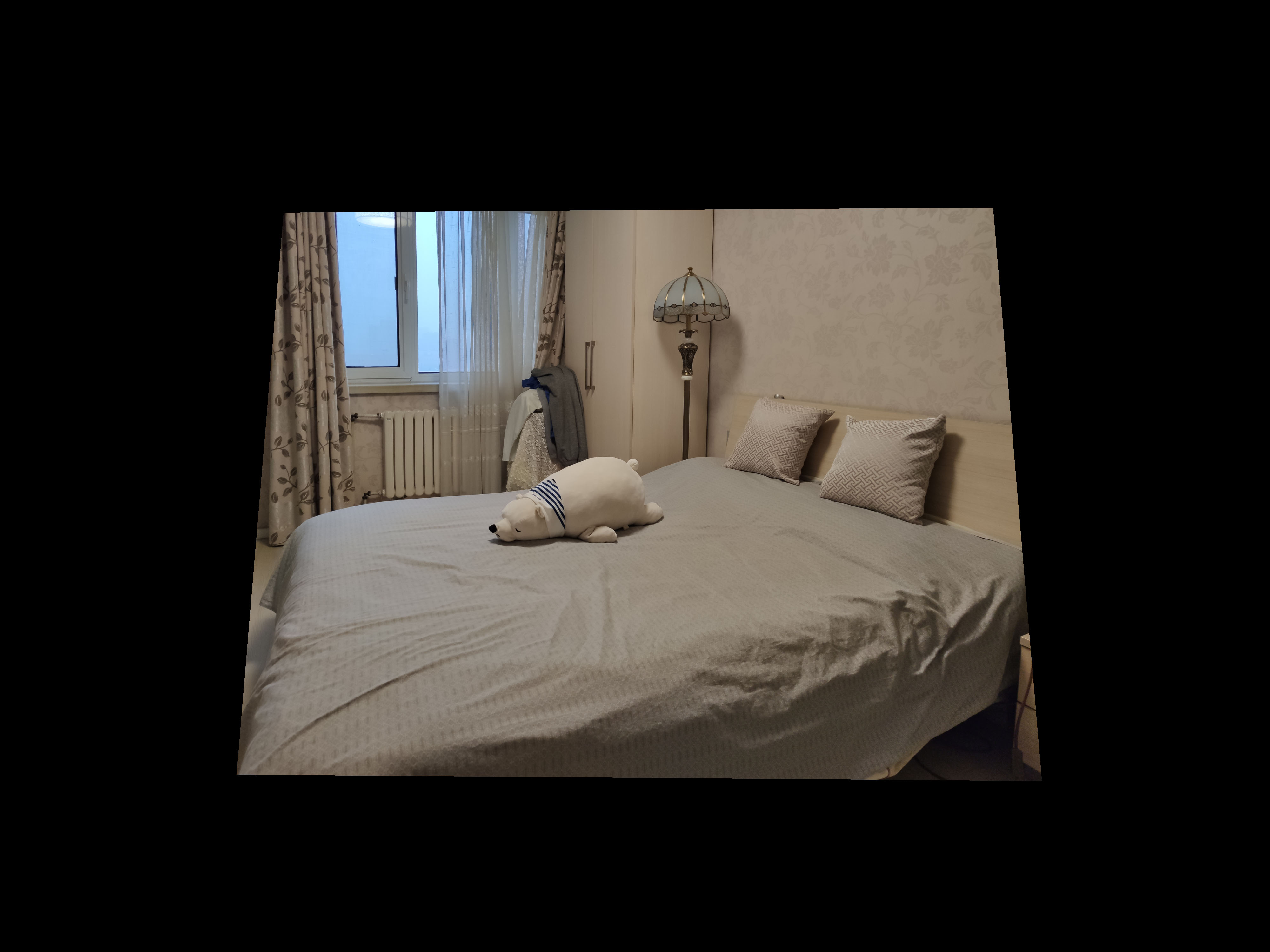
2.4 Image Rectification
Once we warped the image, we would have a rectified picture. We can rectify images and create frontal-parallel or ground-parallel
views of images without using any novel data.
I recovered the homography by computing the projective transformation matrix, H, between the two sets of points. Then, I used the corrospondences
to setup a system of linear equations and solved using least squares to find the parameters for the homography. This homography then allowed us to compute the transformation on the entire image.
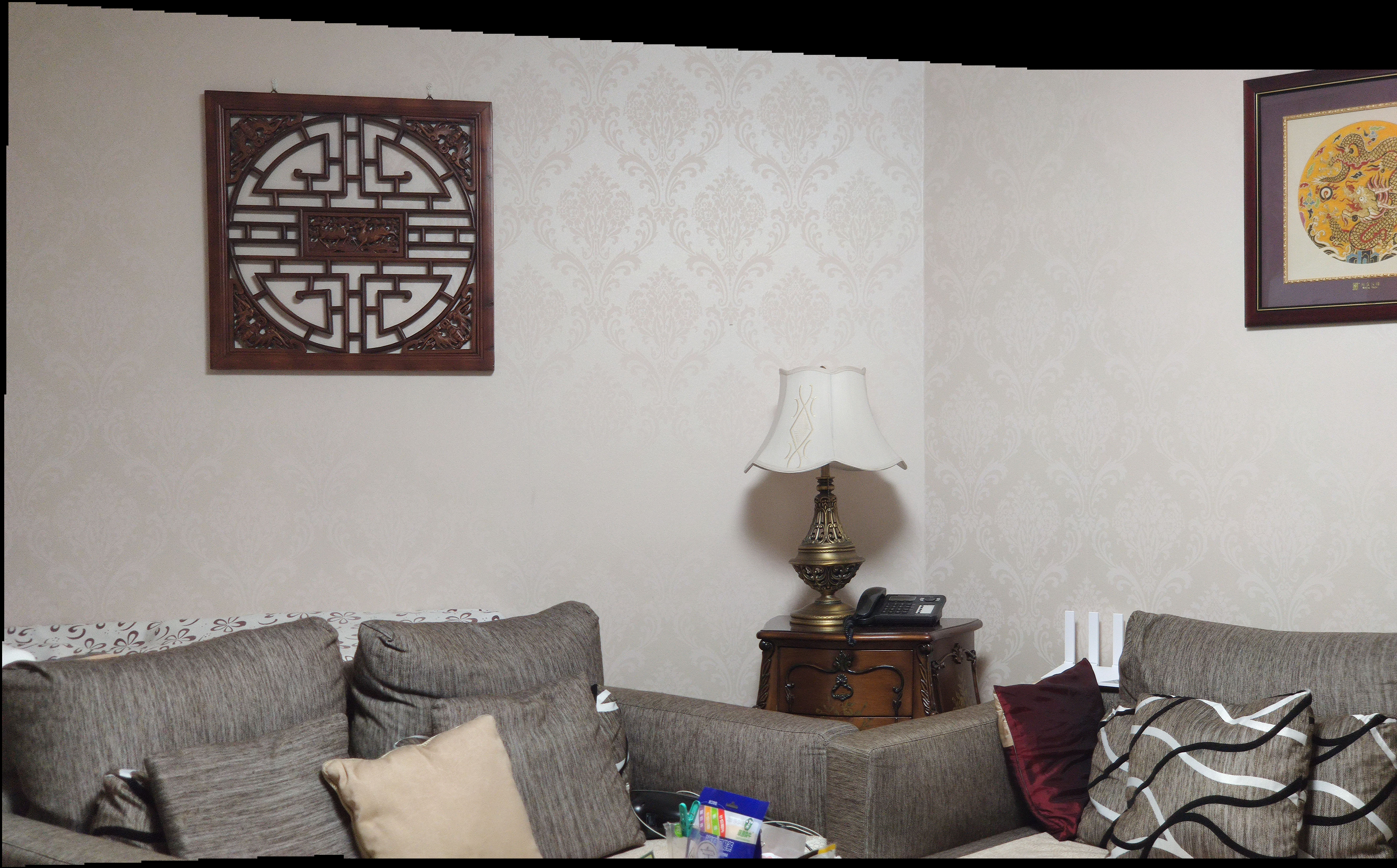
2.5 Mosaic Blending
We finally create digital mosaics and panoramas by stitching together pairs of images. I used alpha calibration blending.
The results are the following:
2.6 What I learned
First, I familarized myself with homography. When I took the Introduction to Robotics class, I once utilized it to transformed the image taken from
the robot's wrist camera. Now, after implementing the function by myself, I noticed it is powerful but not mathematically complicated.
Second, I was surprised at how accurate image rectification can really be, and especially how it can be used to view shapes and drawings from completely different angles,
offering new perspectives on elements of our visible world!
3 Auto-Stitching
For part B of the project, I implemented feature matching for auto-stitching images into a mosaic. The implementation is composed of Harris interest point detector,
adaptive non-maximal suppression, feature description extraction, feature matching, and 4-point RANSAC for homography computation. I finished the implemenation
with the guidance of the paper Multi-Image Matching using Multi-Scale Oriented Patches.
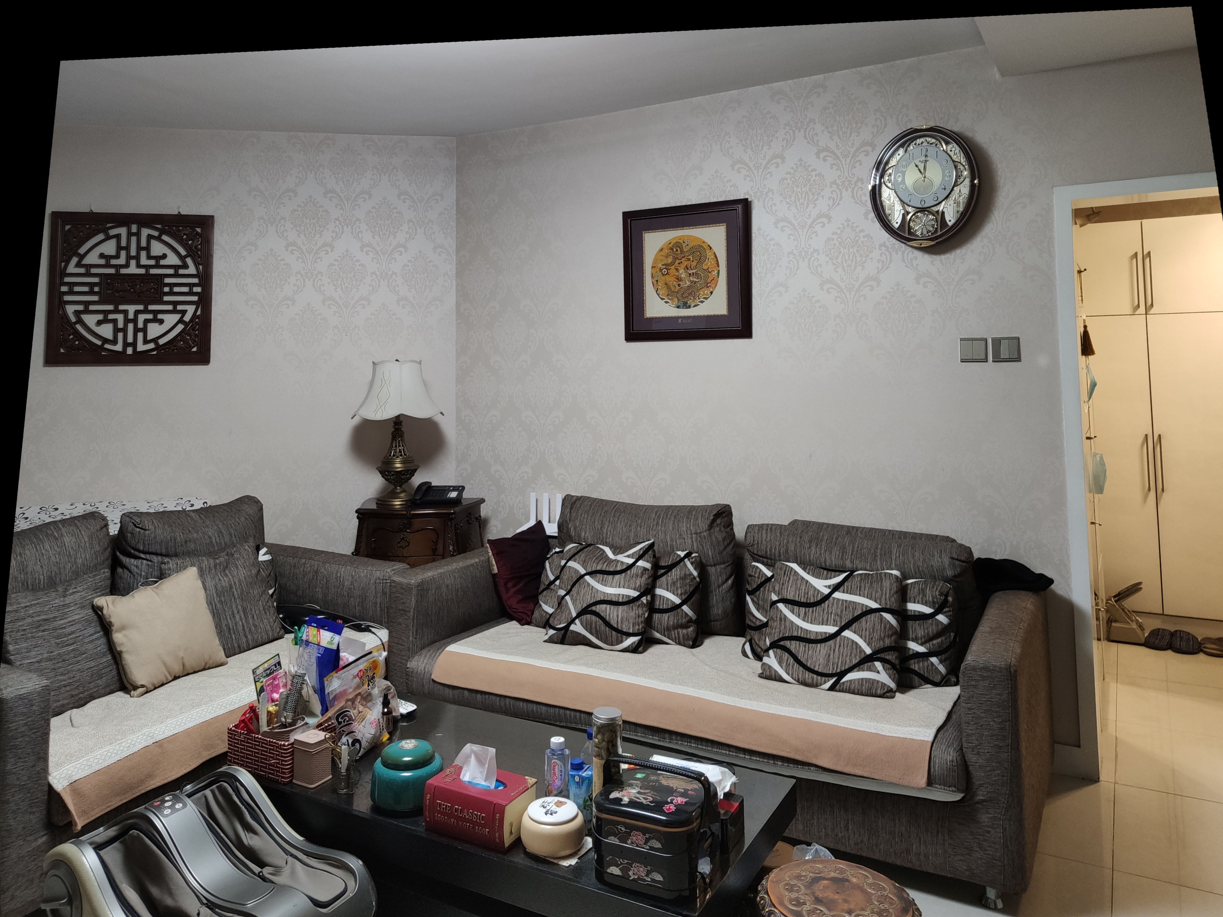
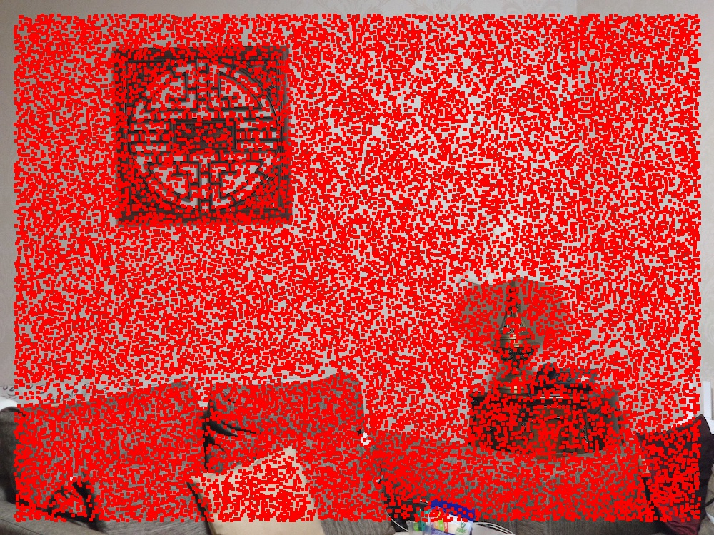
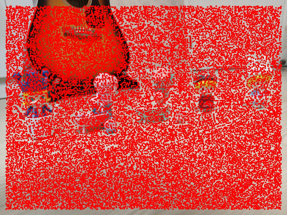
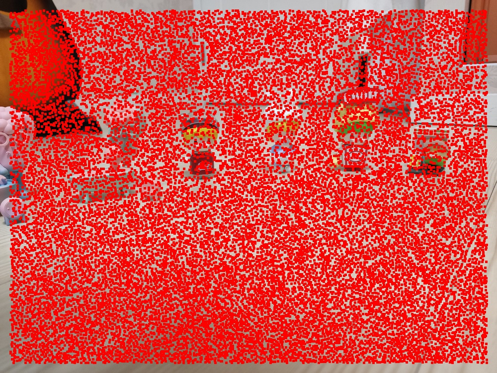
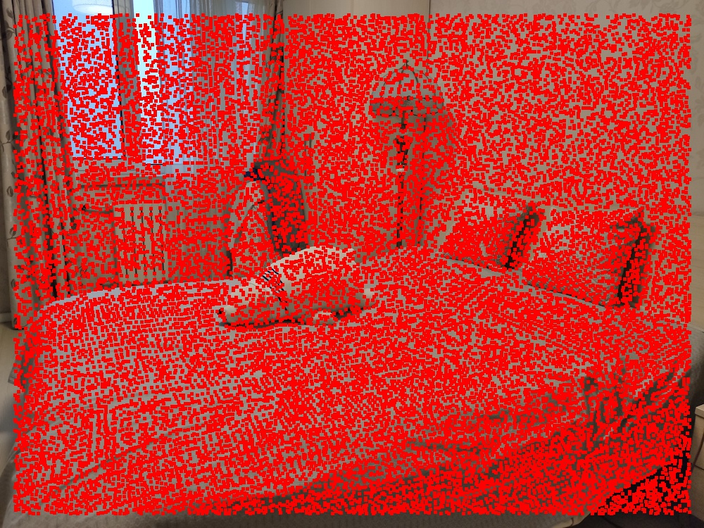
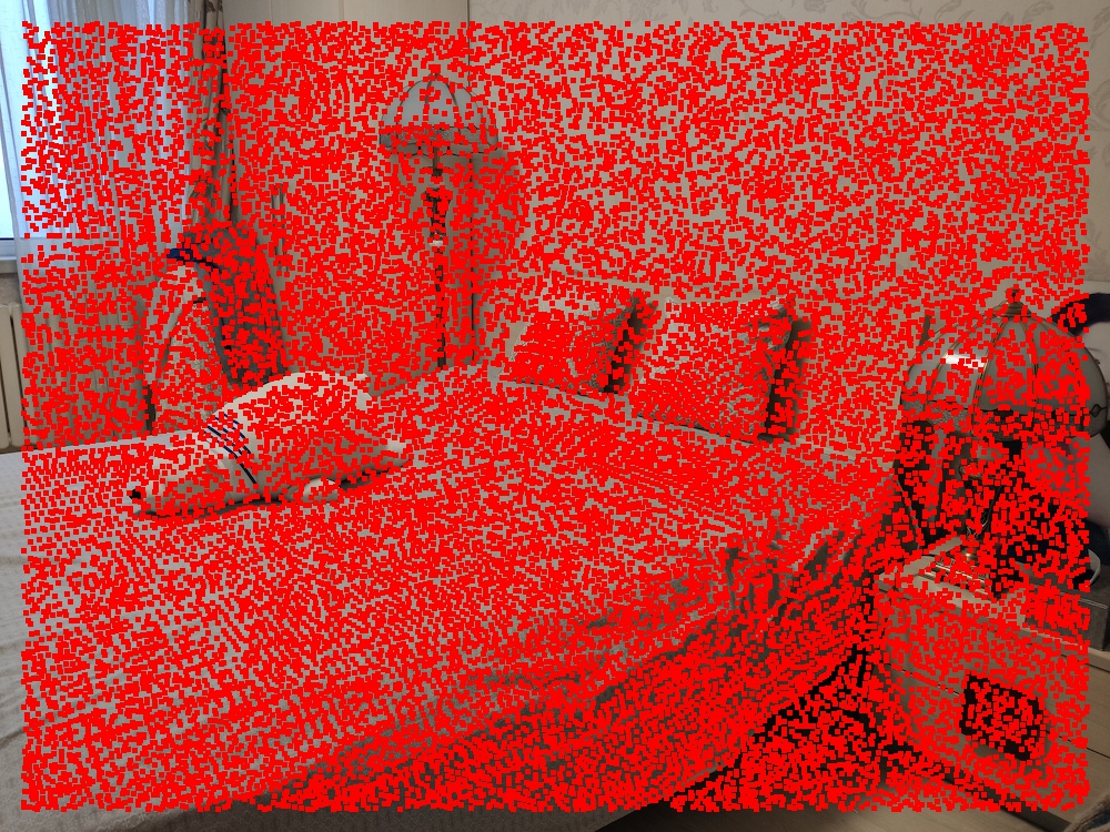
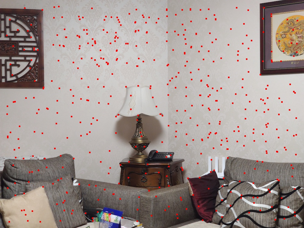
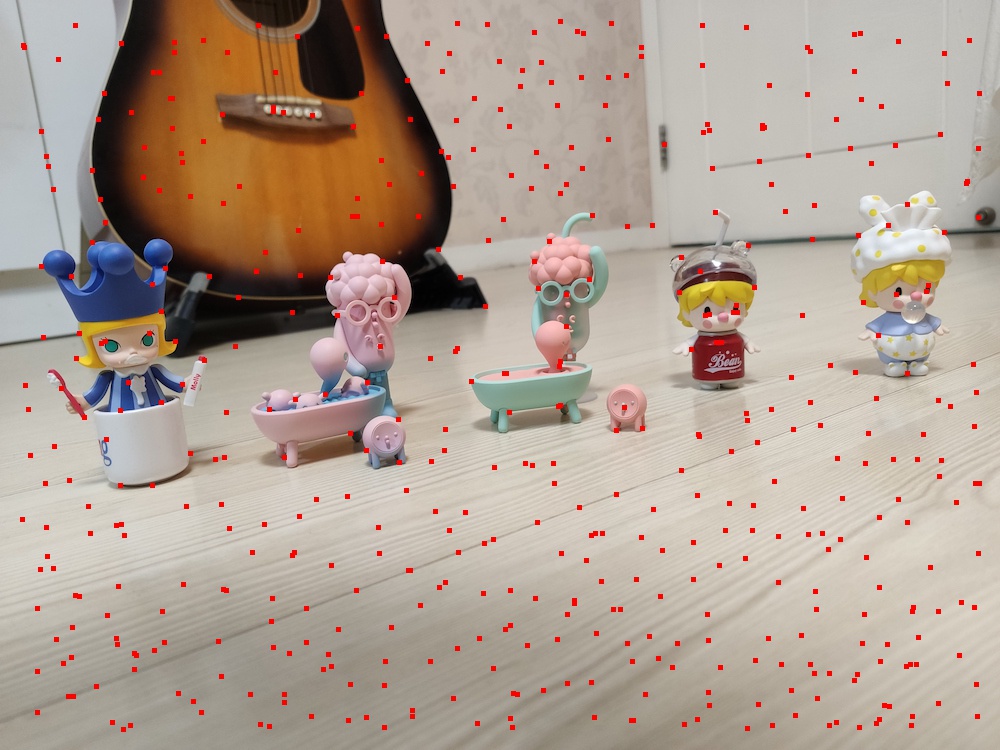
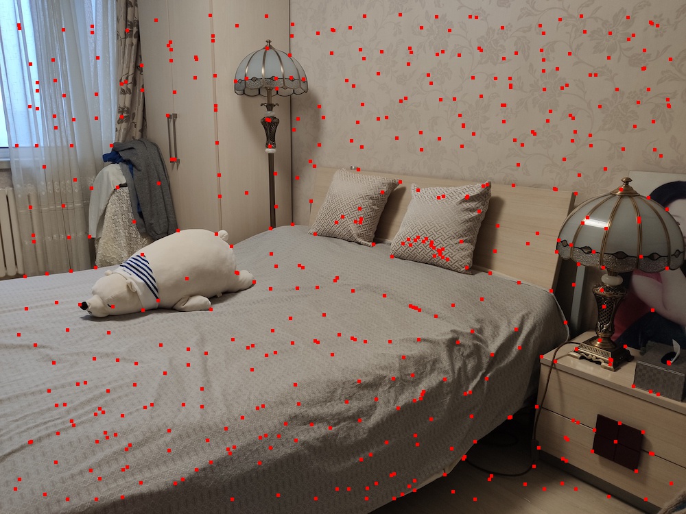
3.0 Interest Point Detection
The interest points we use are multi-scale Harris corners [1, 2]. I used min_distance=1 so the results contain a large number of points. Below are the Harris interest points for our picture frame images.
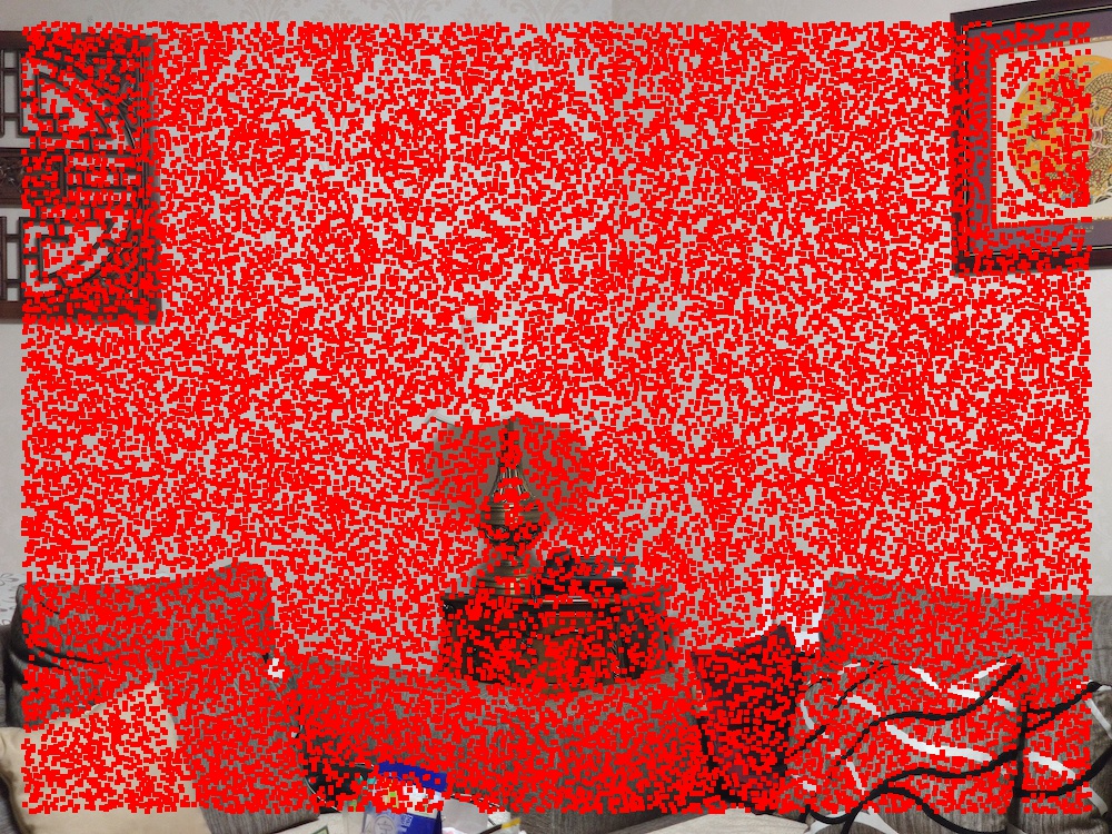
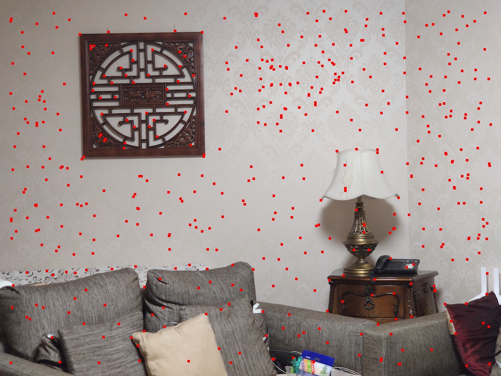
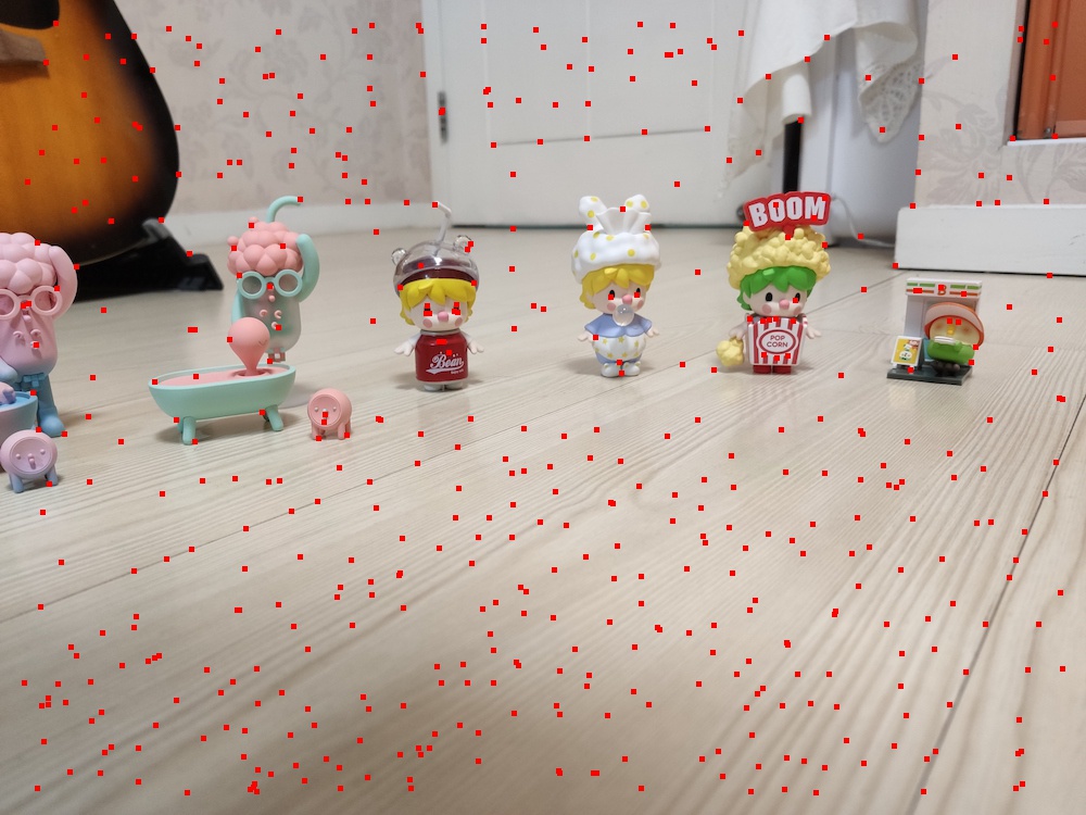
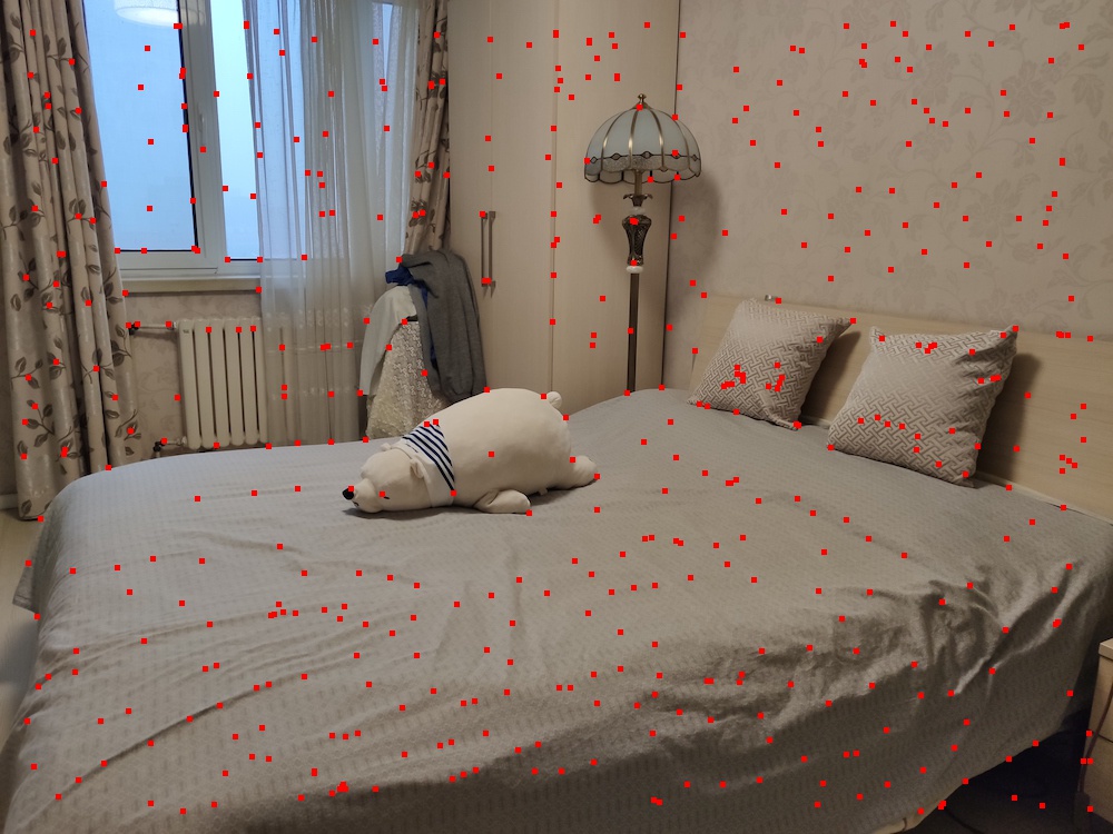
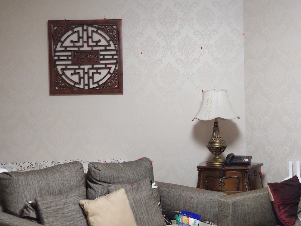
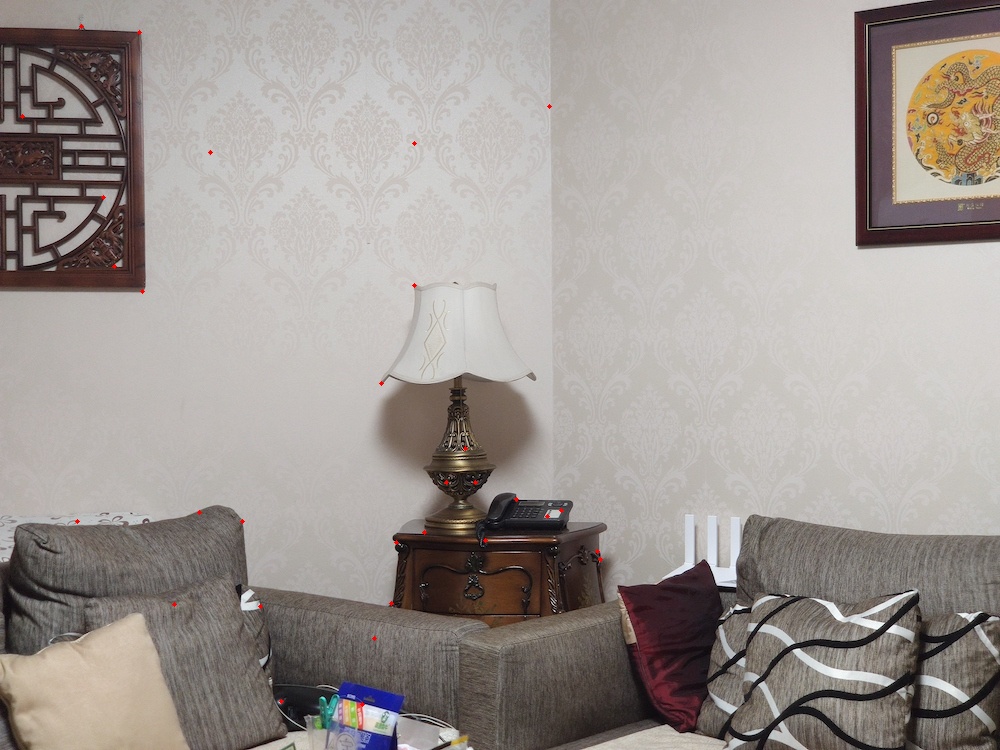
3.1 Adaptive Non-Maximal Suppression
Below is the suppressed Harris Interest Points. As can be seen, the amount of points has been substantially reduced, removing the points that have a low corner strength while also keeping a
nice even distribution of points throughout the images.
3.2 Feature Descriptor extraction
Once we have our points between two images, we have to match them together using feature descriptors. I described each point by the 40 x 40 patch around the point. To reduce error due to noise or brightness or other factors, I gaussian blurred the patch and down sampled it to an 8 x 8 feature descriptor. Finally, I subtracted the mean and divided by the standard deviation for each patch.
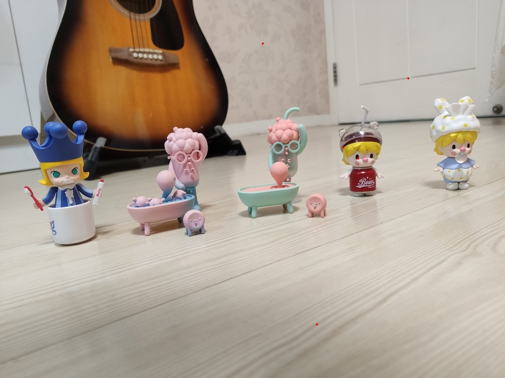
3.3 Feature Matching
Given Multi-scale Oriented Patches extracted from all images, we are going to find geometrically consistent feature matches between all images. I looked at each interest point in one image, and compare the distance between its feature descriptor and the feature descriptor of every interest point in the other image. I kept track of the minimum distance and the 2nd-to-smallest distance from the patch in the source image to every patch the destination image. If this ratio of the minimum distance to the 2nd-to-smallest distance is small enough, then I included it as a pair of matching features.
3.4 RANSAC - Computing a Homography
We now have a map of correspondences and need to compute the morph. I then used the random consensus sampling algorithm or RANSAC to find the best set of points. First, I randomly selected 4 points from my array of points and calculated the homography for these points. I used it to warp the left image points into the right image points. Afterwards, I calculated the Euclidean distance between random transformed points to the actual points of the right image. I repeated this process for about 1000 iterations and at the end selected the homography that gave me the largest set of inlier points. We can run RANSAC.
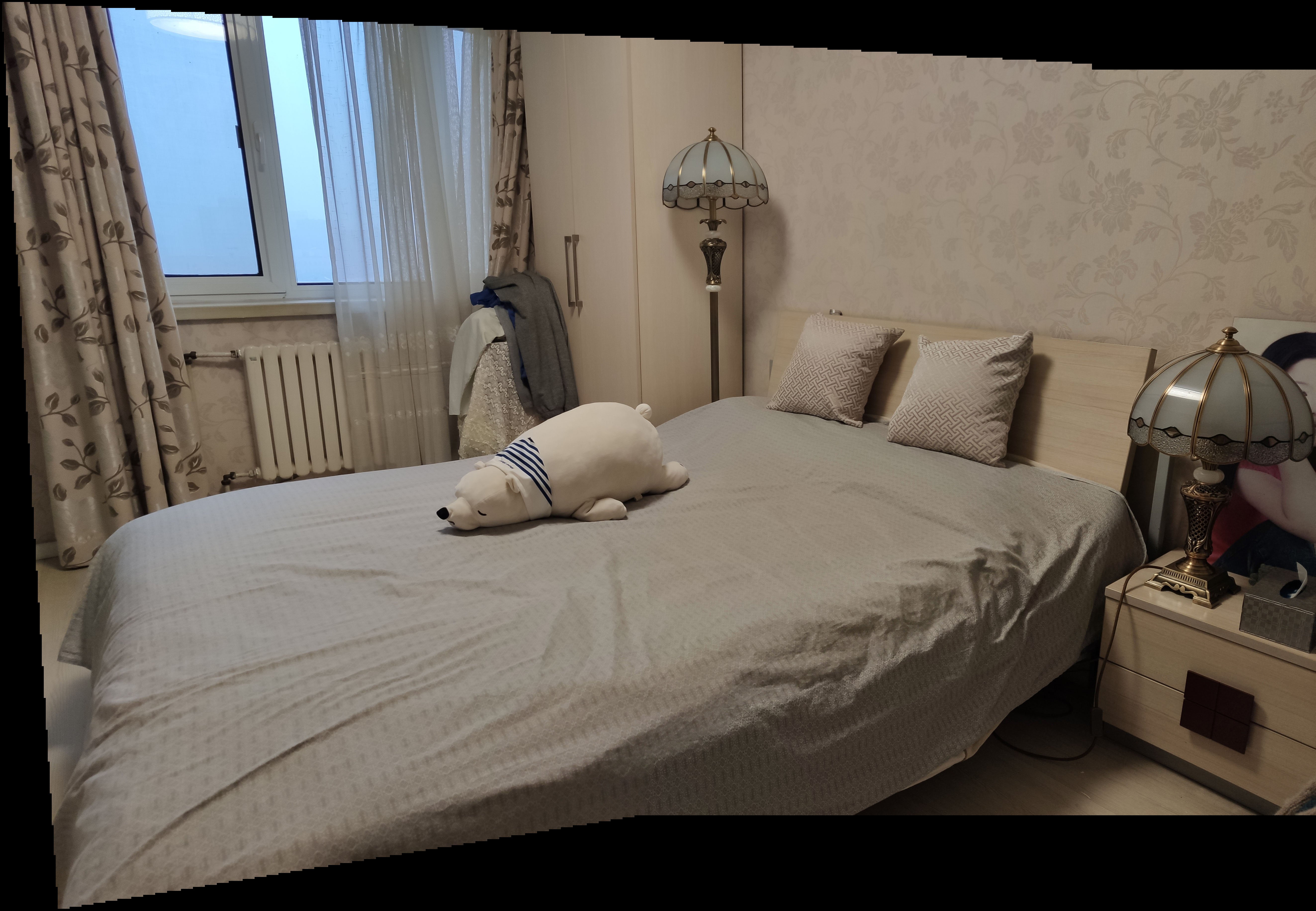
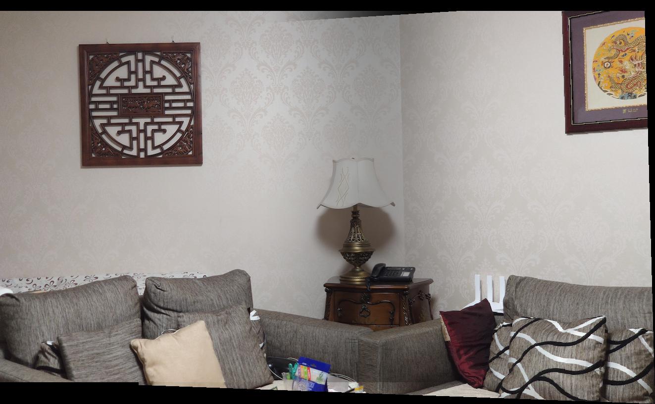
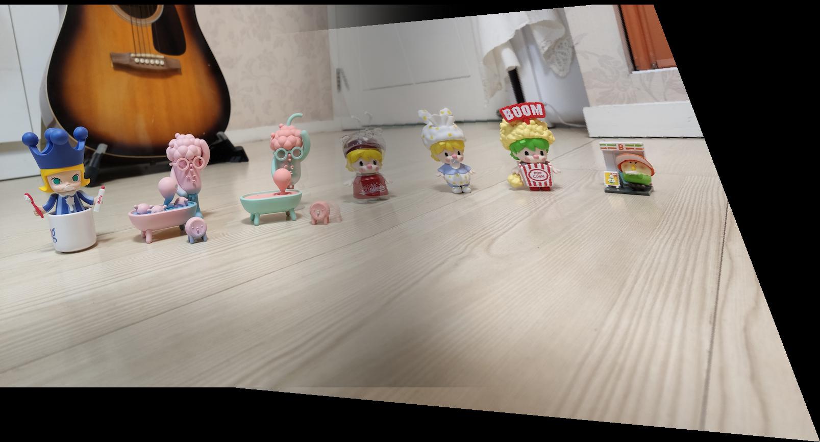
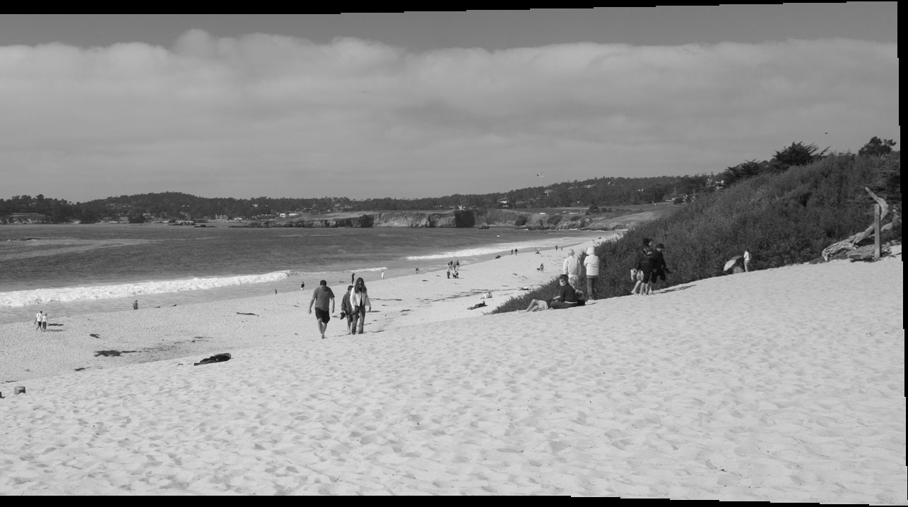
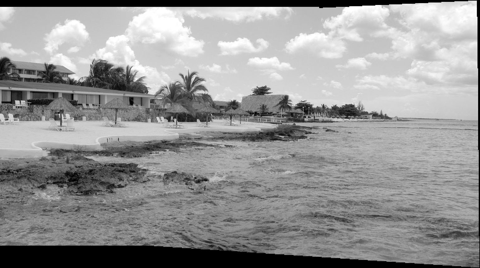
3.5 Stitching a Panorama
The below images are the mosaic image that was created with manual correspondence points and the mosaic image that was created with our automatic correspondences. The left are the manual selected results from Part A, and the right are the auto selected results. As the images show, the manual selected results are better than the auto-stitched results.
4 What I Learned
I really enjoyed working on the part B of this project. Panorama is a function that I used a lot for photography. I think it’s amazing how something as simple as corners can be used to identify real objects such as tables, couches, carpet designs and more. If I had more time, I would like to use machine learning methods to detect the features.