CS194-26 Project 5: Homography and image stitching
Kevin Shi
Overview
In this project, I will write stitching algorithms for panoramas from scratch.
Part 1: Manual Point Choosing
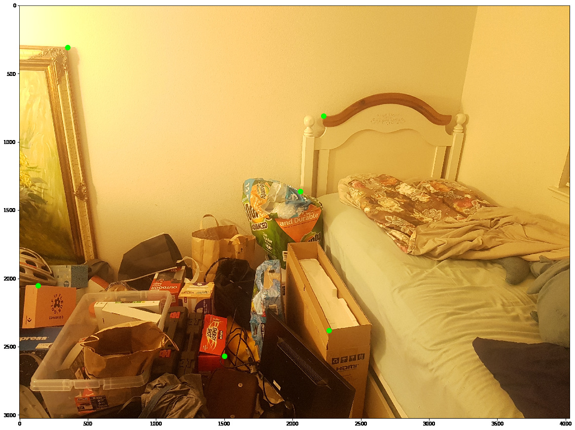
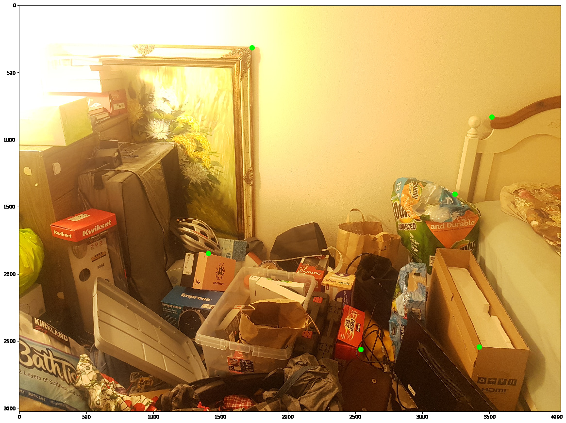
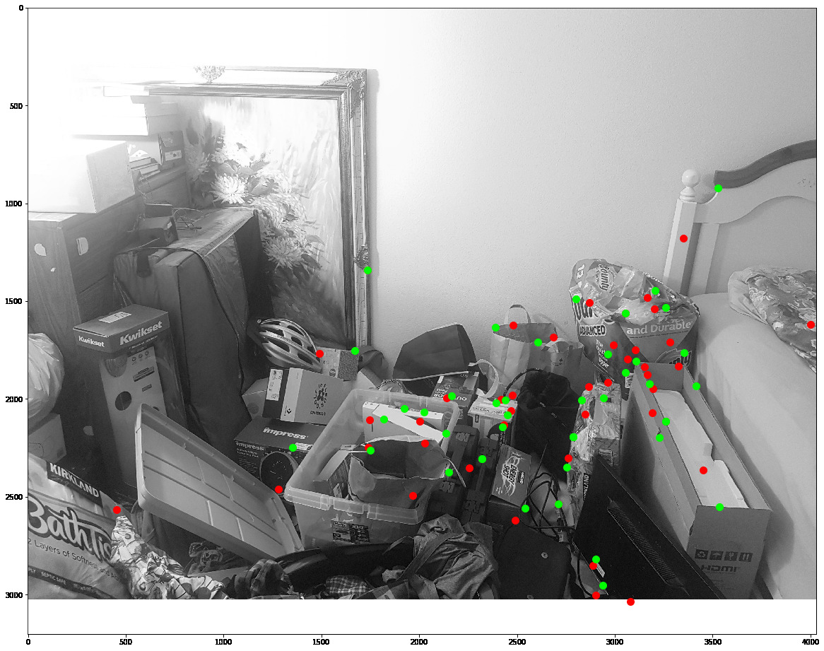
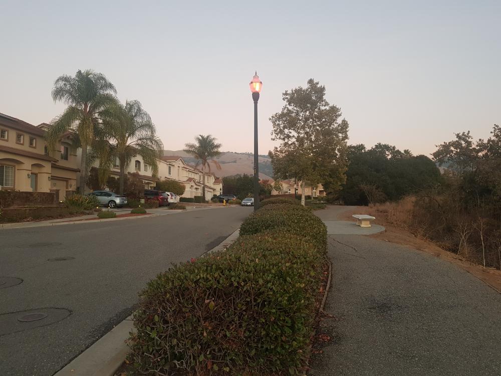
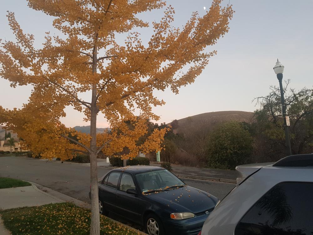
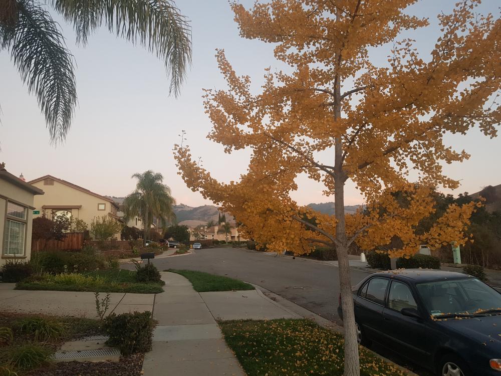
We must first start with an image to stitch. In this first part I will stitch images by manually choosing points, calculating the Homography, and finally warping and stitching.
Here are the images and the points I chose. You can see that I chose corners because they are the easiest to match accurately.
Part 1.1: Homography
We will calculate a Homography matrix to warp the images. In theory, since Homography maticies only have 8 unknowns, so we only need 4 points. However, it is better to leave room for error, so as you can see in the images above, we choose more points. This leads to a overdetermined equation that I use least squares to solve. Hopefully the error in manual choosing of points can be modelled by a gaussian, in which case the gaussian noise will converge to the optimal solution with least squares.
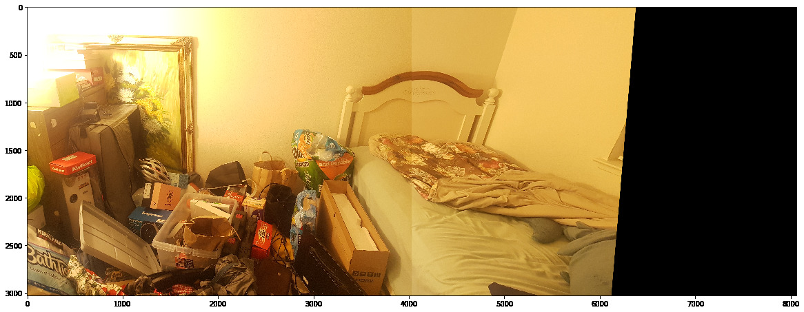
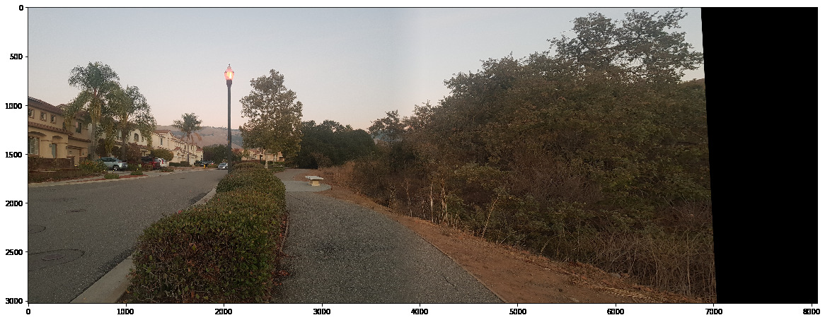
We first use this homography transform to get a "bird's eye" view of the room. Let's see whats in the box.

Part 1.2: Warp and stitch
Now let's use the points and warp our image to match.
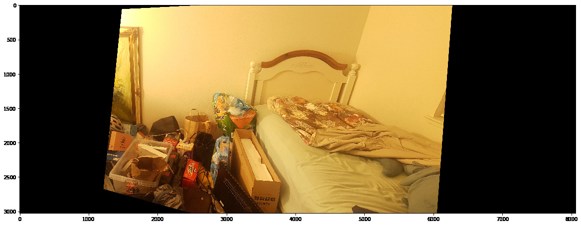
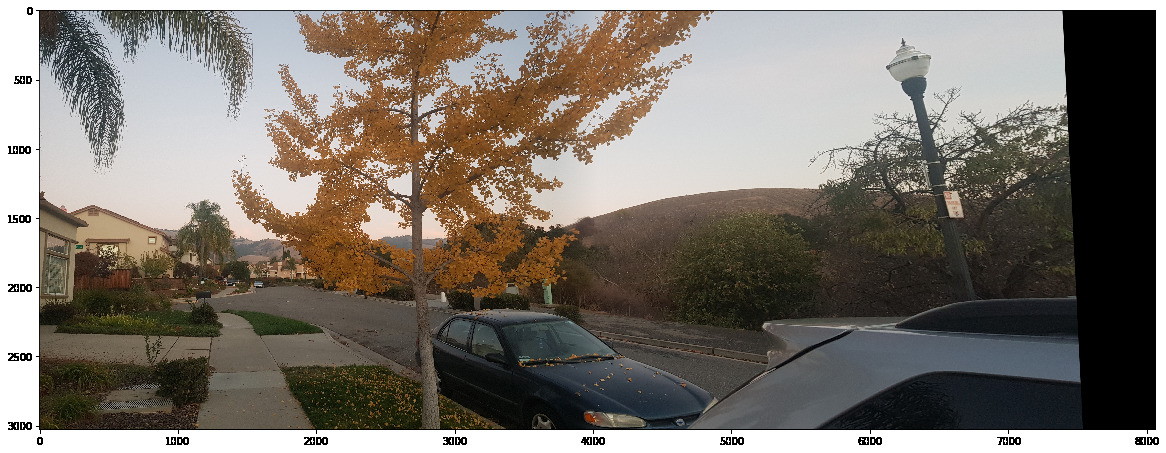
Now if we just naively stitch them together by lying the images ontop of each other, we get a rough panorama:

However, that seam is quite ugly, lets fix it by using a weighted average based on distance from the seam.
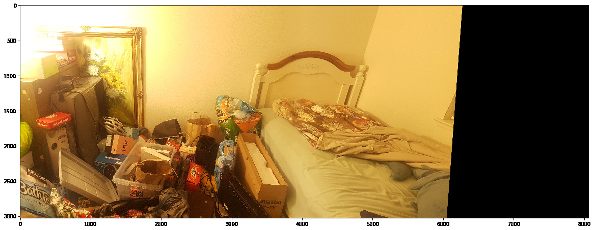
That looks much better! Now we have a panorama algorithm given two images and corresponding points.
Part 2: Auto Point Choosing
Now that we have homography stitching, let's attempt to find these points automatically. We will use feature matching, specifically, the MOPS algorithm.
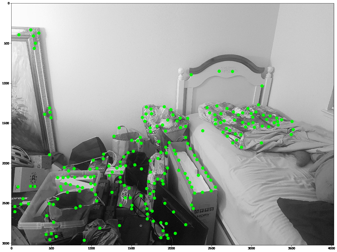
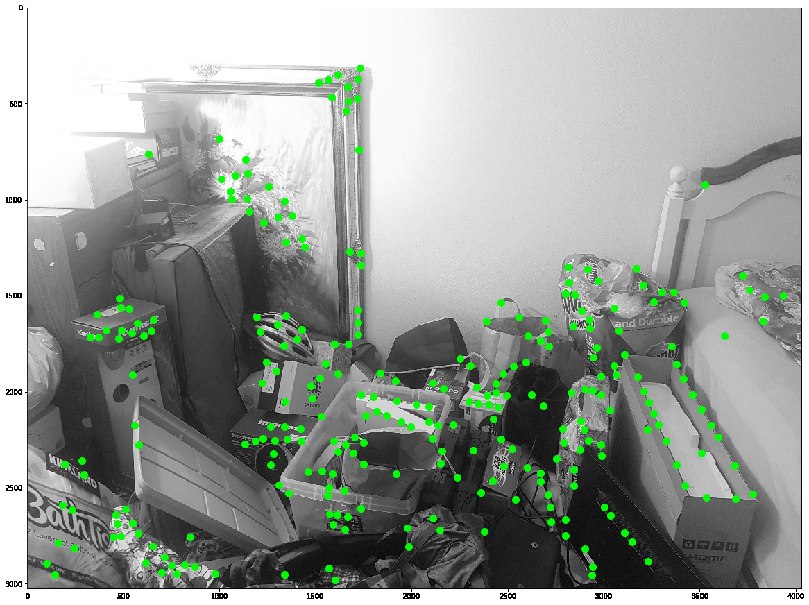
Part 2.1: Harris Corner detection
We will first use the Harris Algorithm to find features in the image. Specifically a Harris Feature is where the derivative of the frame has large changes in any direction, meaning that we have a corner. This yields far too many points of interest, most of which are redundant or non-interesting. Thus, we need to implement adaptive non-maximal suppression to find significant features. Here is the result:
Part 2.2 MOPS Feature Extraction
The features we will be choosing are the MOPS features. The features are rather simple, a normalized max-pool of the area around the feature will be our descriptor. Here is an example of one of our features and it's corresponding descriptor.


Part 2.3 Feature Matching
Then it's not too difficult to find the nearest neighbors using l2 distance (SSD). We find the two nearest neighbors in the image we want to warp.

However, we can see that these points are poor matches. We can use Lowe's Ratio test to filter these matches based on the observation that good match pairs have much better first neighbor distance than second neighbor distance.
Here is a good match:
First our source feature and descriptor
Then our first and second neighbors

We can see pretty obviously that the first descriptor is much closer to our source than the second. We can also see that the match for the first neighbor is very good. Compared to the previous example, there is a much larger difference in our 2 neighbors
Part 2.4 RANSAC
Now that we can match features, we can match them using homography; however, this will lead to a poor homography because OLS is very sensitive to ouliers, and even with our ratio test, we still may have bad matches.
The solution is to use RANdom Sample and Consensus. This algorithm consists of random sampling of points, warping based on this random sample, then counting the "Consensus" by the number of inliers(warped points within their respective match + a predefined margin), or in other words, the matches that agree with this random sample.
This will lead to bad and good matches:

Then we have good homography matches, so we can put it altogether and auto stitch two images
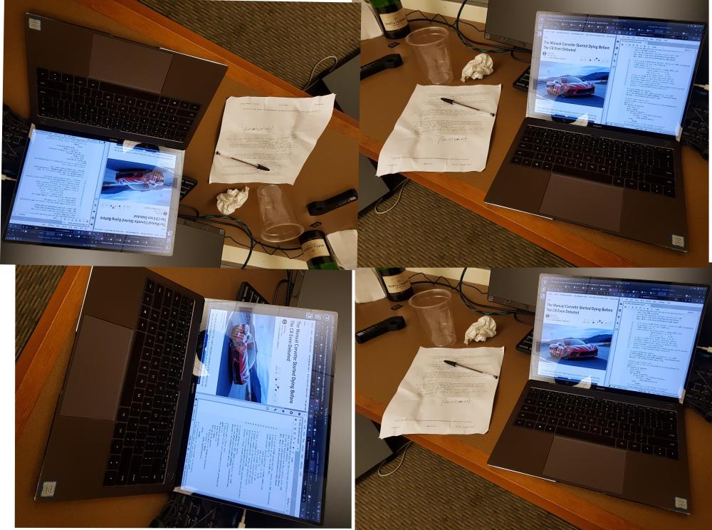
Let's not use any blending and compare the manual and auto stitching
Pretty good! Now let's see the blended image as well as some other images

This one I accidentally left auto exposure on, so we have two images with different exposures, but the algorithm still performed.

I've worked with feature detectors on a high level before, but it was very interesting to actually learn how they work and how to implement them.
Side Project with Homography and Features
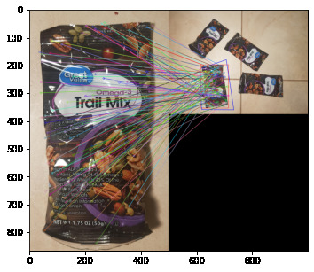
This project is to find matching objects in an image given a source image. I use the opencv features and homography to make the base of the project easier. I chose ORB feature descriptors for this project because in my tests it worked just as well as SURF and SIFT in this application, and using patented algorithms leads to a bad taste in my mouth. It is easier to show the results of the algorithm rather than just explaining, so here's an example:


Selective Search
First I use selective search to find potential objects. Selective search was an algorithm first pioneered for R-CNNs and works by first dividing the pixels of an image into a graph, then grouping conservatively (graph-based segmentation). Than it groups these segmented graphs based on similarity heuristics: color, texture, size, amd shape.
Basic Cutoff
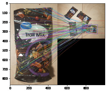
We match points in each of the bounding boxes using crosscheck as our matching algorithm. Crosscheck is a simple matching algorithm where we only keep the point if the matches are both each others' mutual nearest neighbors. I originally attempted this with Lowe's ratio test; however, even with a low cutoff, the ratio test did a subpar job. I think this is because the bounding boxes are large, and thus have multiple of the object in one of the bounding box, leading to neighbors on two different instances of the same object, which leads to similar distances, meaning that Lowe's ratio test fails.
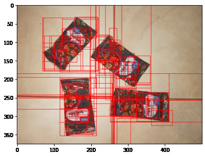
As you can see in the image above, there are way too many potential objects. We thin the herd through a simple cutoff bounding boxes that have too little matches.
Homography
These bounding boxes are poor representations of the actual object, so we find new bounding boxes using the original image and a homography calculated through the matching points and RANSAC.
Here are the new bounding boxes:
As well as some of the paired bounding boxes and homography:

Homography Angle Cutoff
Some of these new homography boxes obviously are not objects. Here, based on the assumption that the bounding boxes should be well-formed and close to parallelograms, we prune some of the boxes based on the interior angles of the homography box.
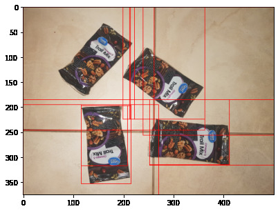
This yields something that actually looks like it is a bounding box
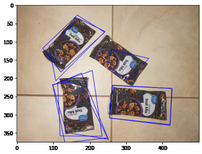
We can see that it's still not the best though, and there seems to be a problem when the objects are too grouped up. This problem is due to the implementation of selective search. Although selective search is based off graph segmentation, which has no concept of bounding rectangles, most implementations of selective search will return a bounding rectangle that is aligned with the x and y axis of the image. This causes boxes to include multiple objects if they are not aligned with the image and are too close together. Perhaps in the future we can add selective search implementation to return a opencv mask and thus not have the problem of this. A quicker and more dirty solution would be to rotate the image 45 degrees and do the process again, after which we would merge the two answers with NMS, which we will discuss in the next section.
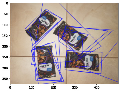
Non-Maximal Suppresion (NMS)
We can see there are many bounding boxes on the same object. We use NMS here to discard boxes that have too much overlap. This requires scoring the boxes to see which is more likely to be the better representation of the object. After many iterations, I settled on a score based on an linear combination of how well-shaped(interior angle) the box was and the number of feature matches. This leads to our final image:
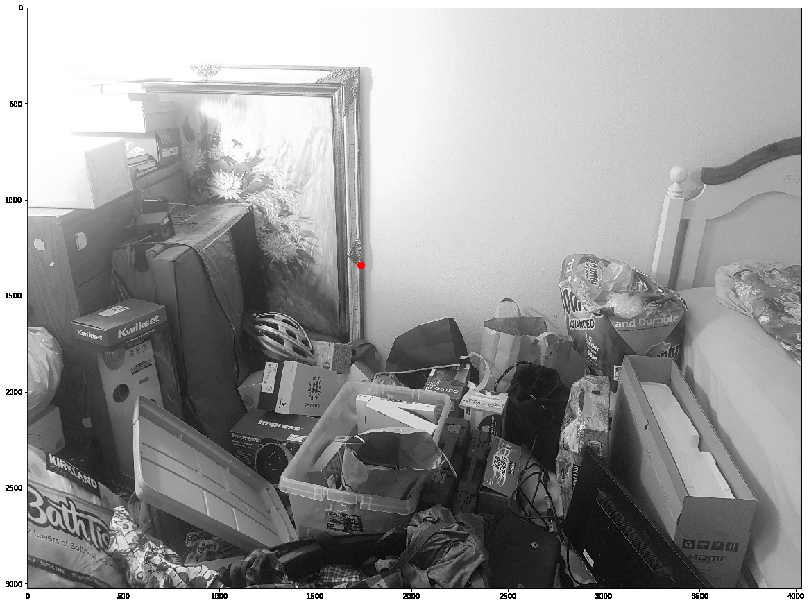
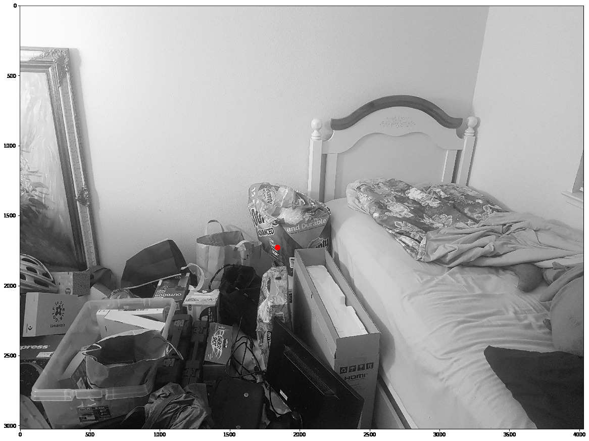
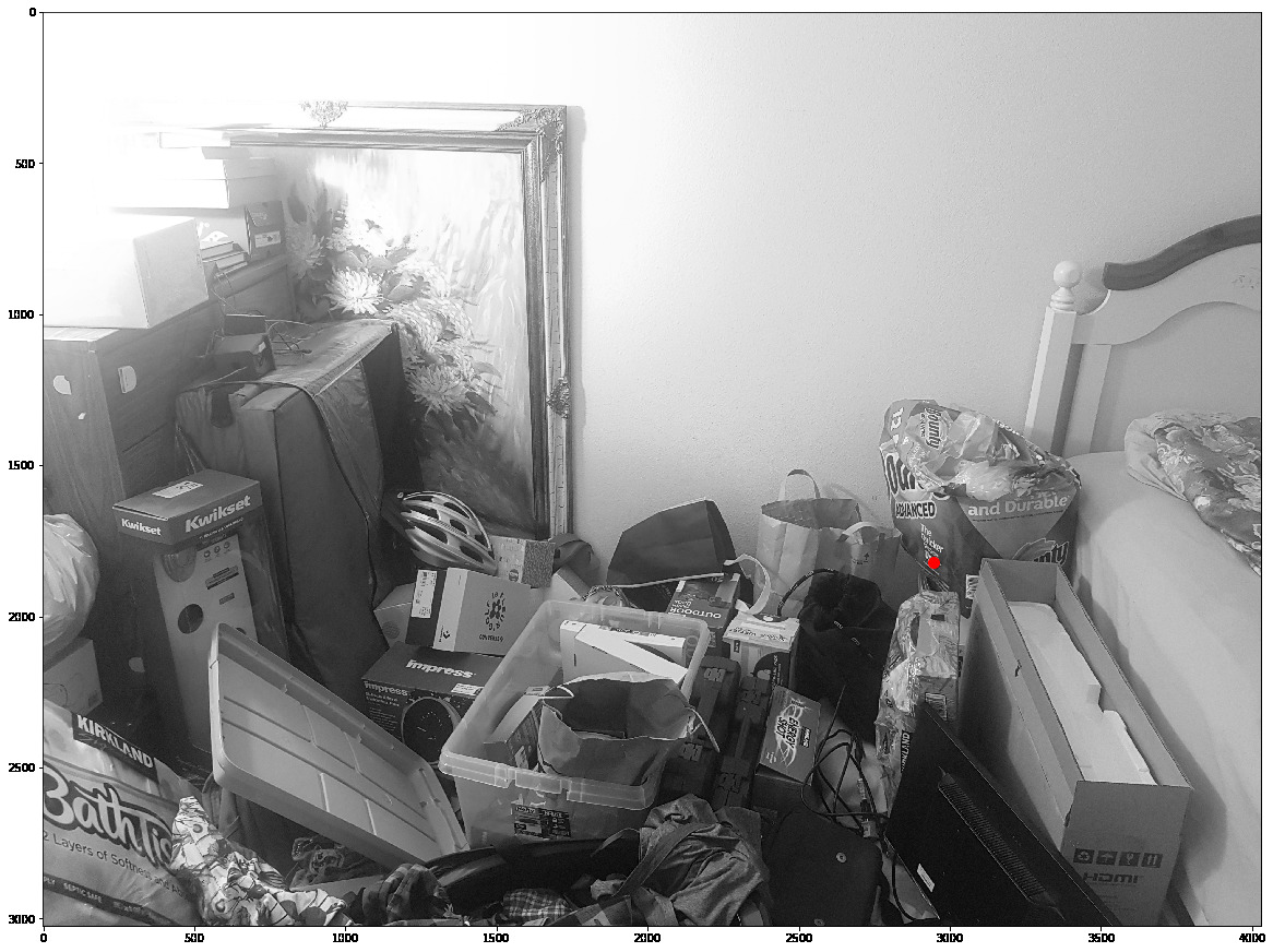
Works in noisy environments
Even with multiple