| image 1 | image 2 |
|---|---|
|
|
|
|
|
|
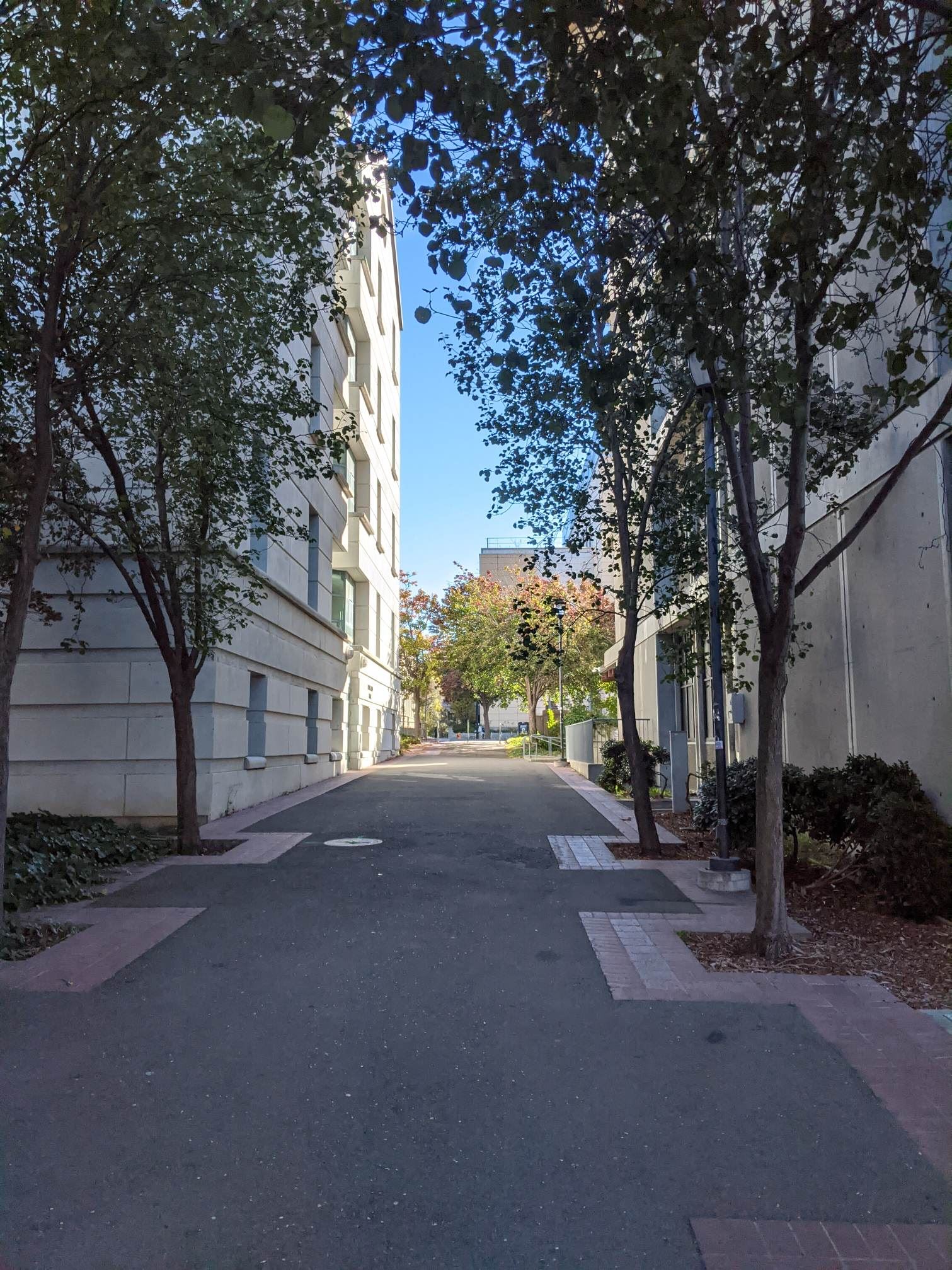
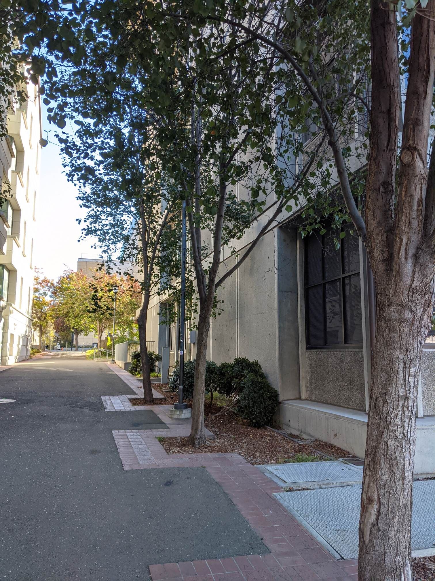
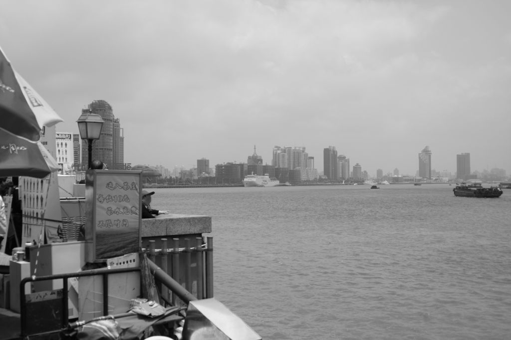
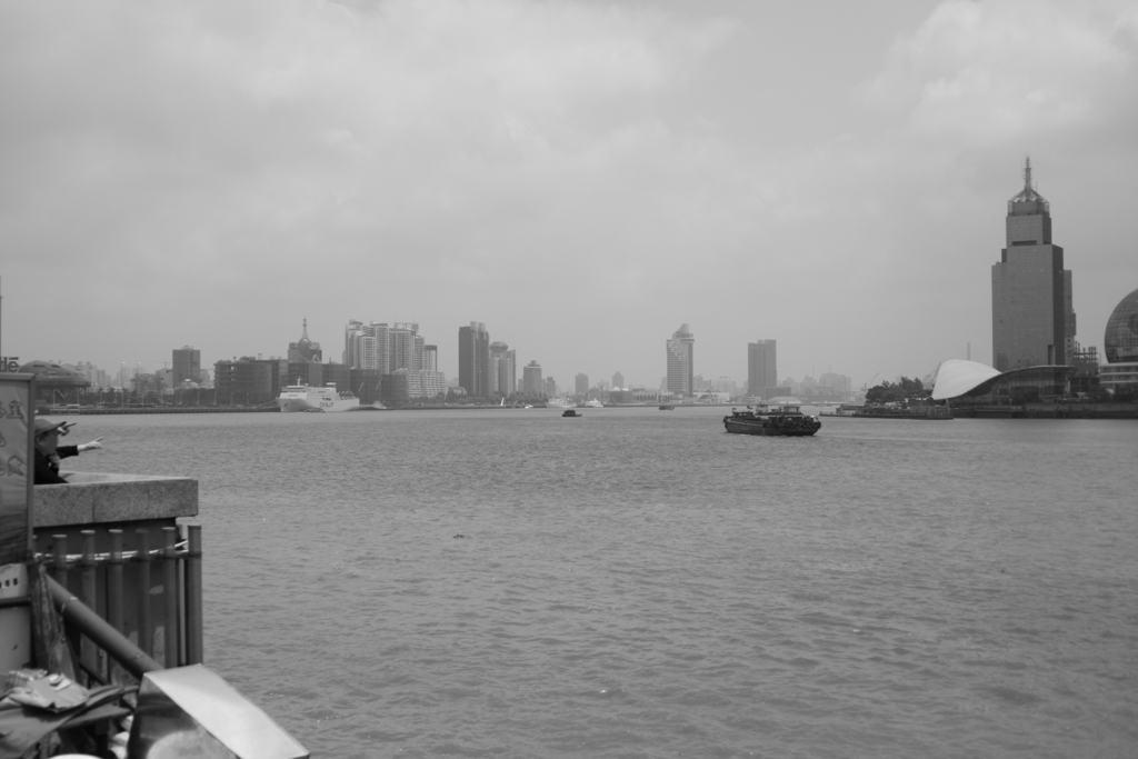
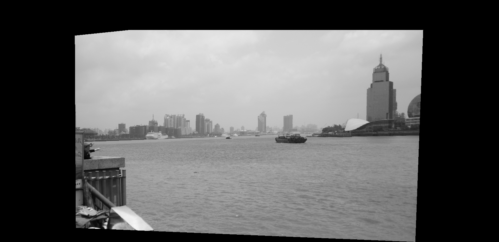
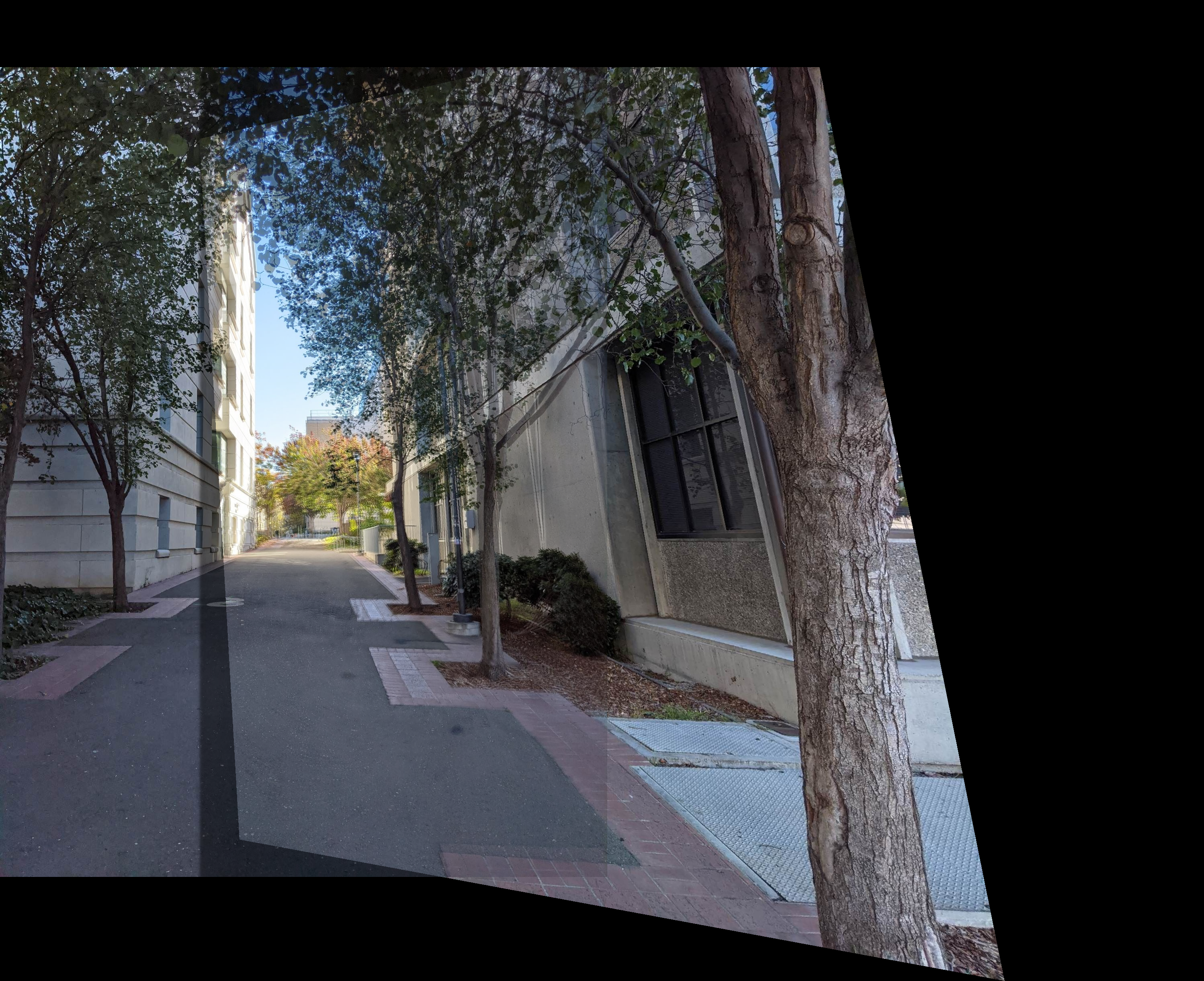
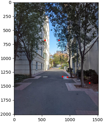
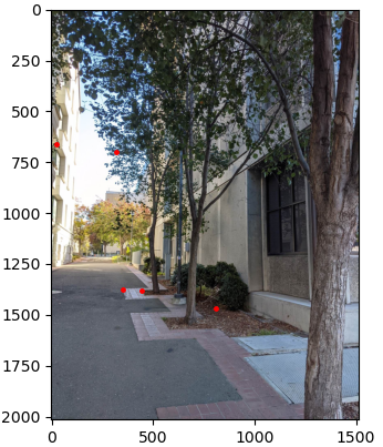
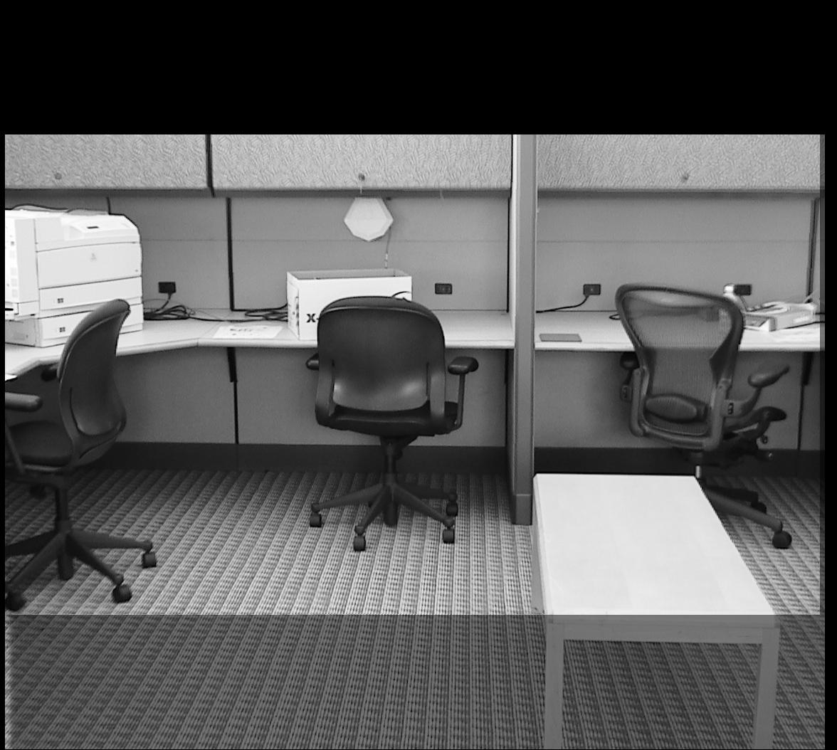
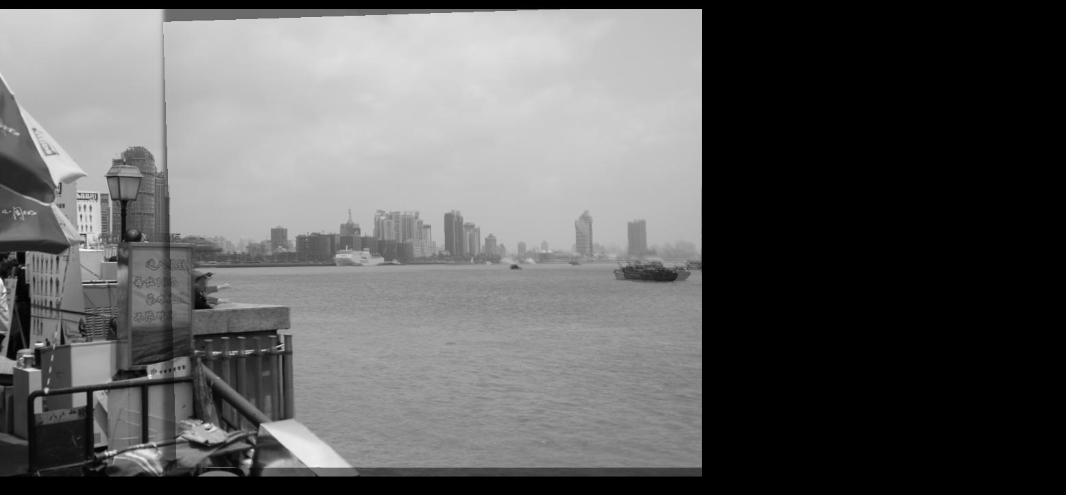
The goal of this project is to stitch together many images to form larger composite images.
I took some pictures of the road between Barker Hall and Koshland Hall on campus and used those for warping. I also found some other image sets online and tested with those.
| image 1 | image 2 |
|---|---|
|
|
|
|
|
|
|
|
|
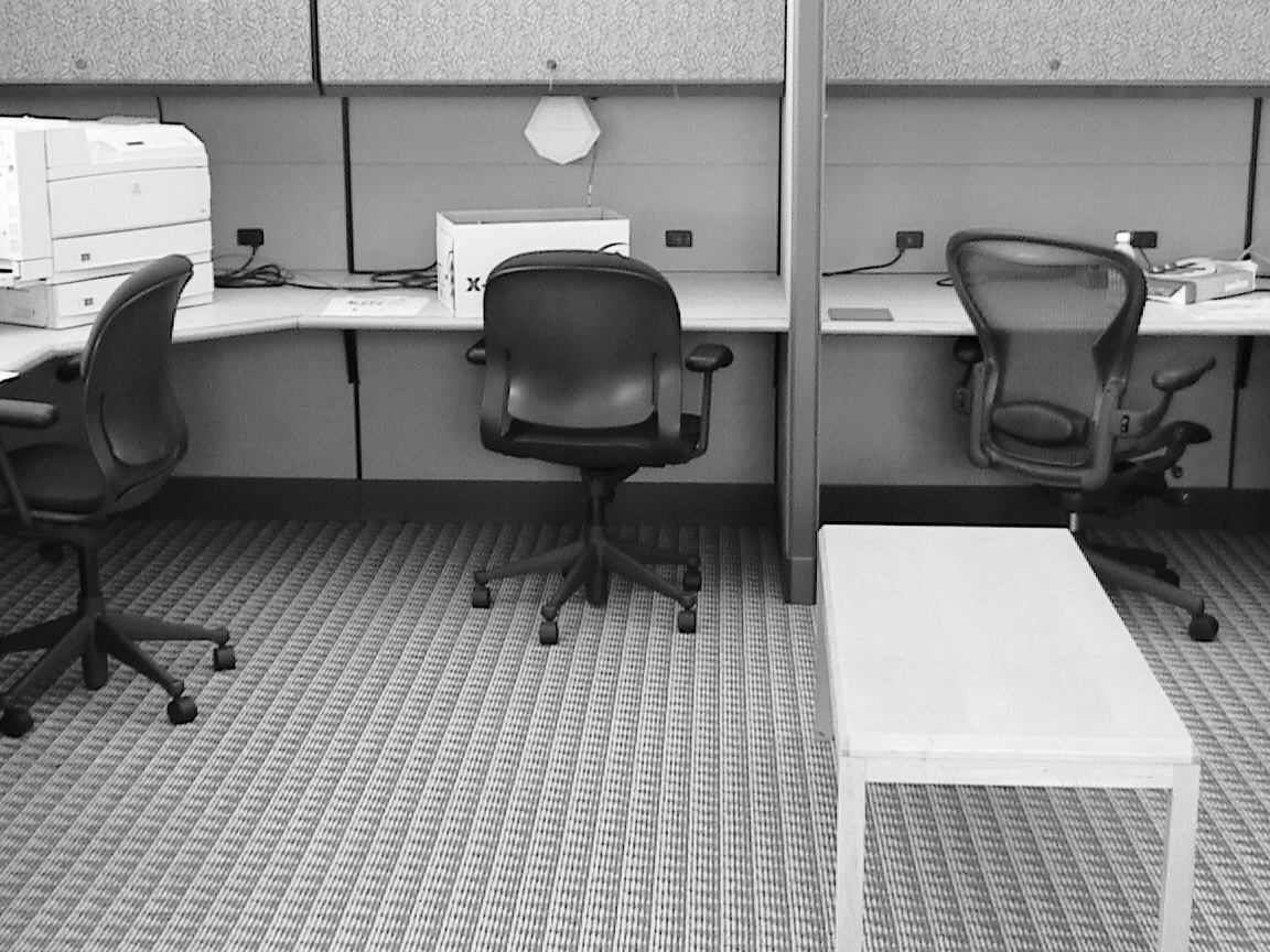
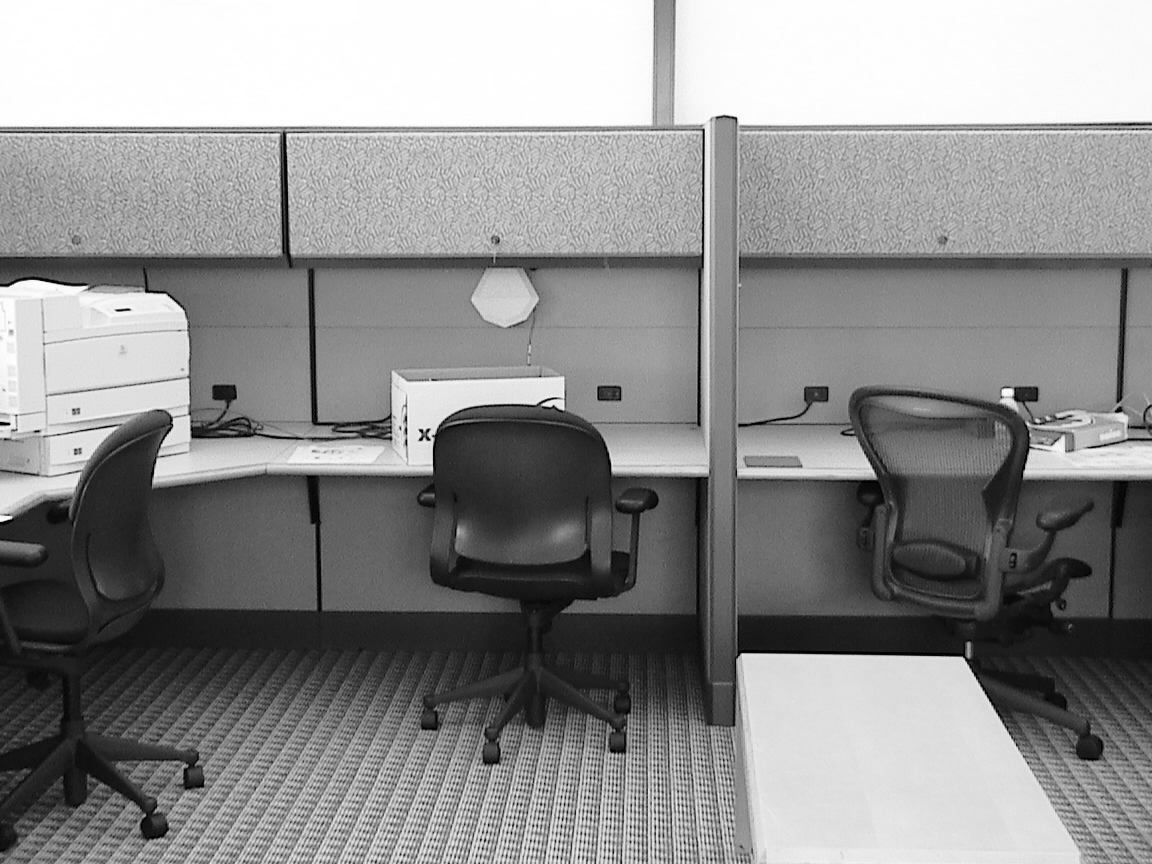
I calculated the honeography matrix H using the equations described in the textbook, Szeliski p.494-496. I used the equation Ah=b, where b is populated with the chosen coordinates on image 1, the one that other images are being warped into. b is a column matrix of the form [x1, y1, x2, y2 ... xn, yn]. A is made up of a stack of

for each coordinate pair, where (x, y) are coordinates from image 2 and (x', y') are coordinates from image 1. I then use np.linalg.lstsq() to calculate h and construct the homeography matrix H from that.
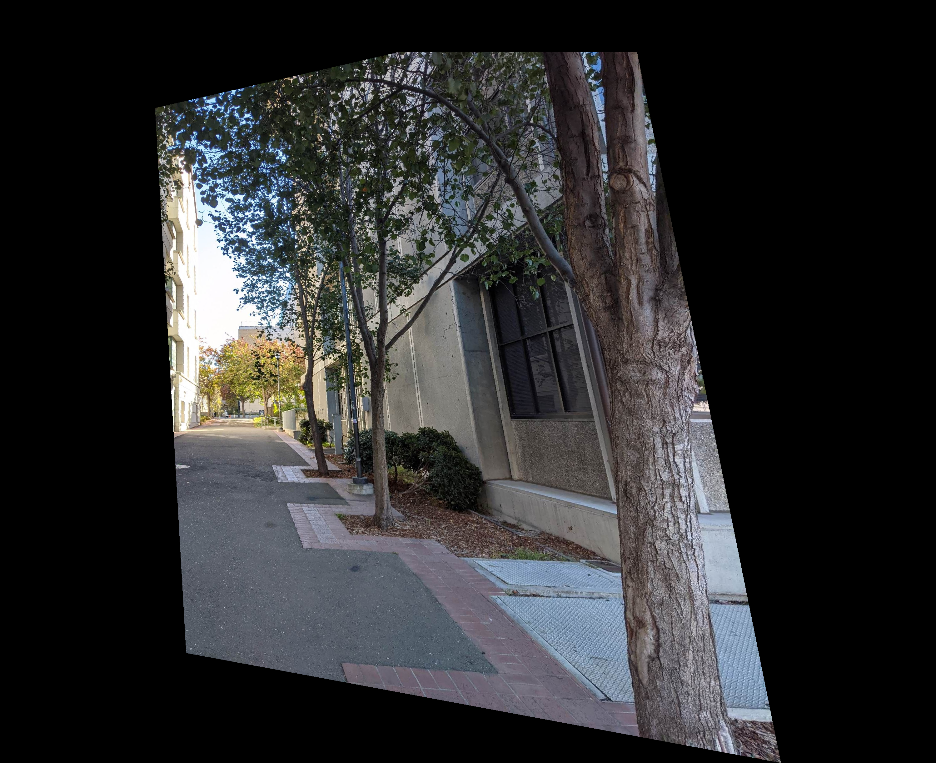
To warp image 2, I need to apply H to the locations of its pixels. I first get the coordinates of the corners, warp them with H, and create a polygon with skimage.draw.polygon() using those coordinates. This polygon is the shape that image 2 will take once warped into image 1's point of view. I create a blank image of zeros and place pixels from the unwarped image 2 into the blank image using the corresponding coordinates from the warped polygon, and that is how I create the warped image.
Warping image 2 as described above gives a rectified image, with image 1 as a reference point.
| image 2 | warped image 2 |
|---|---|
|
|
|
|
|
|
|
|
|
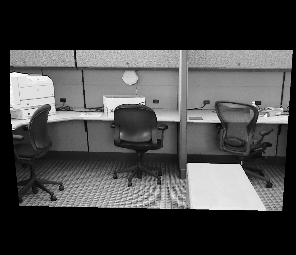
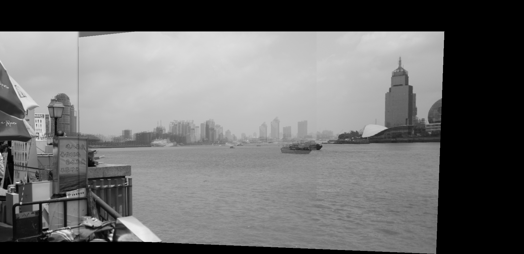
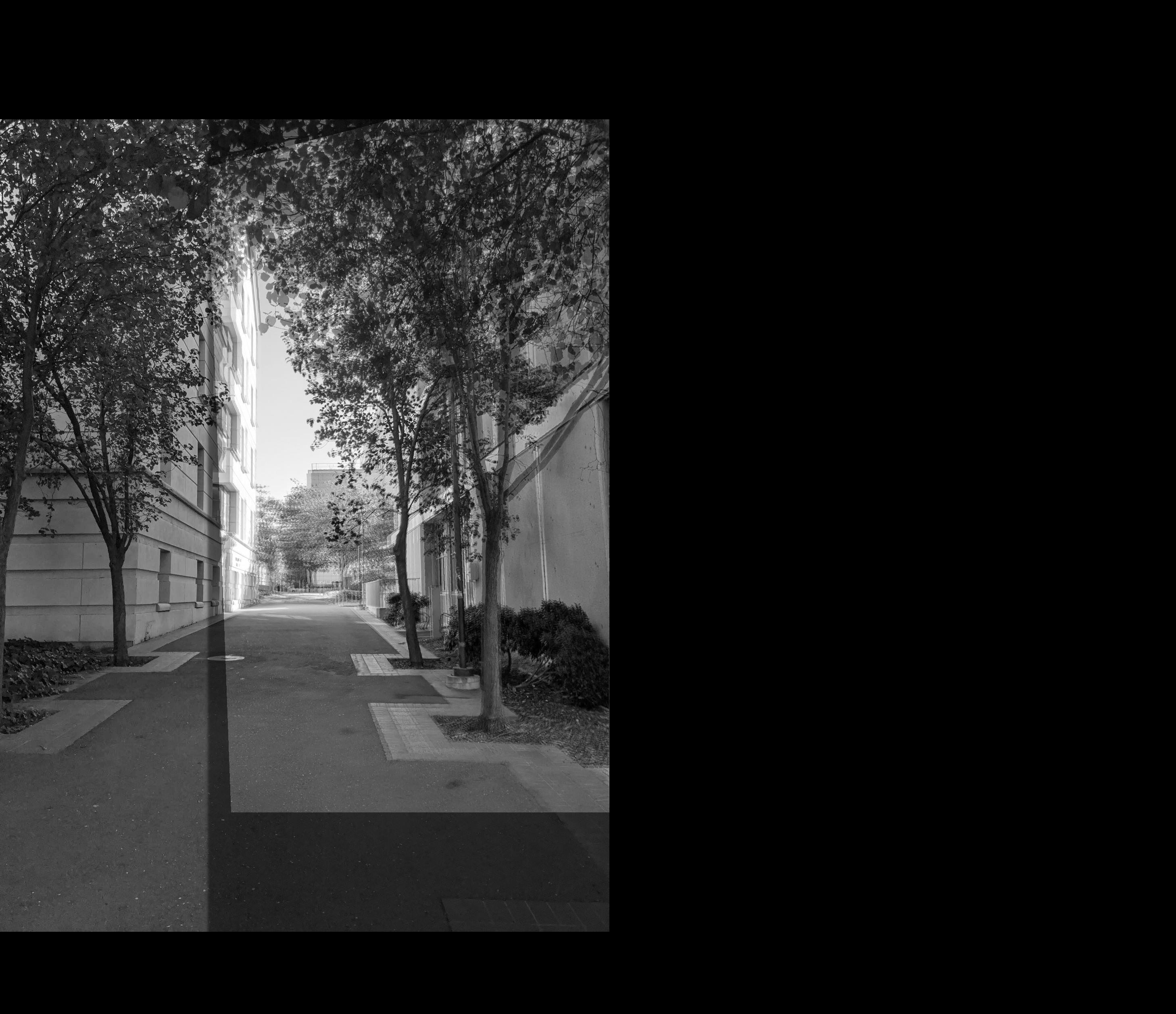
TO blend the images, I created a mask with a sigmoid function that gradually changed from 1 to 0 at some specified threshold. This approach led to a blurring effect where similar features of the blending images didn't align exactly right and you can see the features from both the reference image and the warped image. Additionally, the warped image has large black borders around it, which get included in the blending and lead to some areas getting unnecessarily darkened. The resulting blended images are ultimately still recognizable, they just have extra visual effects.
|
|
|
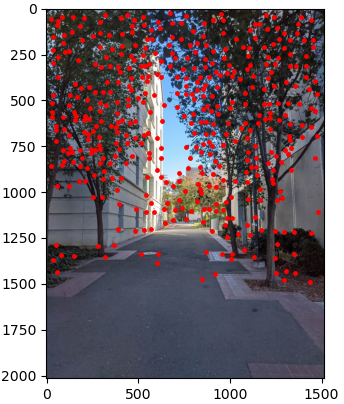
The provided Harris code detects corners in the provided image. Following advice on Piazza, I swapped peak_local_max for corner_peaks and increased min_distance to 20, which resulted in more distinct points with less clutter.
|
|
Detected Harris Corners
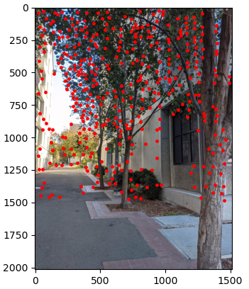
The purpose of Adaptive Non-Maximal Suppression (ANMS) is to restrict the maximum number of interest points from the given image, as well as ensure they are well-distributed over the image, since feature matching takes time and less points means faster matching.
For implementation I calculated the distance from each Harris point to every other Harris point, provided that the corner strength at the source point was no more than 0.9 times the corner strength of the other points, and recorded the minimum distance found. After doing this for each Harris point, I sorted them by radius in descending order and kept the top 500.
The pseudocode provided by Myles Domingo on Piazza was very helpful in understanding what exactly the MOPS paper described and figuring out my ANMS implementation.
|
|
Harris Corners after ANMS
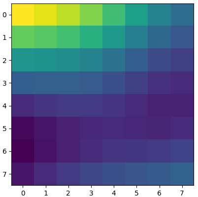
After whittling down the number of feature points in each image, we need to match them, and before matching we need to extract features for comparison. I take a 40x40 window around each feature point and Gaussian blur it into an 8x8 feature descriptor, then normalize it. This does discard any points that would have a window that exceeds the bounds of the image, however.
|
|
Feature Extraction
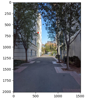
For feature mapping, we have to compare every feature in one image to every feature in the other. I compute the SSD between every pair of feature patches between the two images. Then, for each feature in the first image I check its top two SSDs with the second image's feature patches and make sure their ratio is less than 0.4 (the smallest SSD is at most 0.4 times the SSD of the second smallest). If this is not the case then there is no clear feature match, and the point is discarded.
|

|
|
|
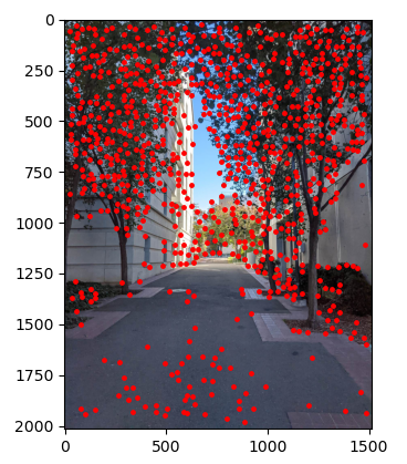
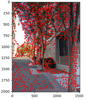
Matching Features
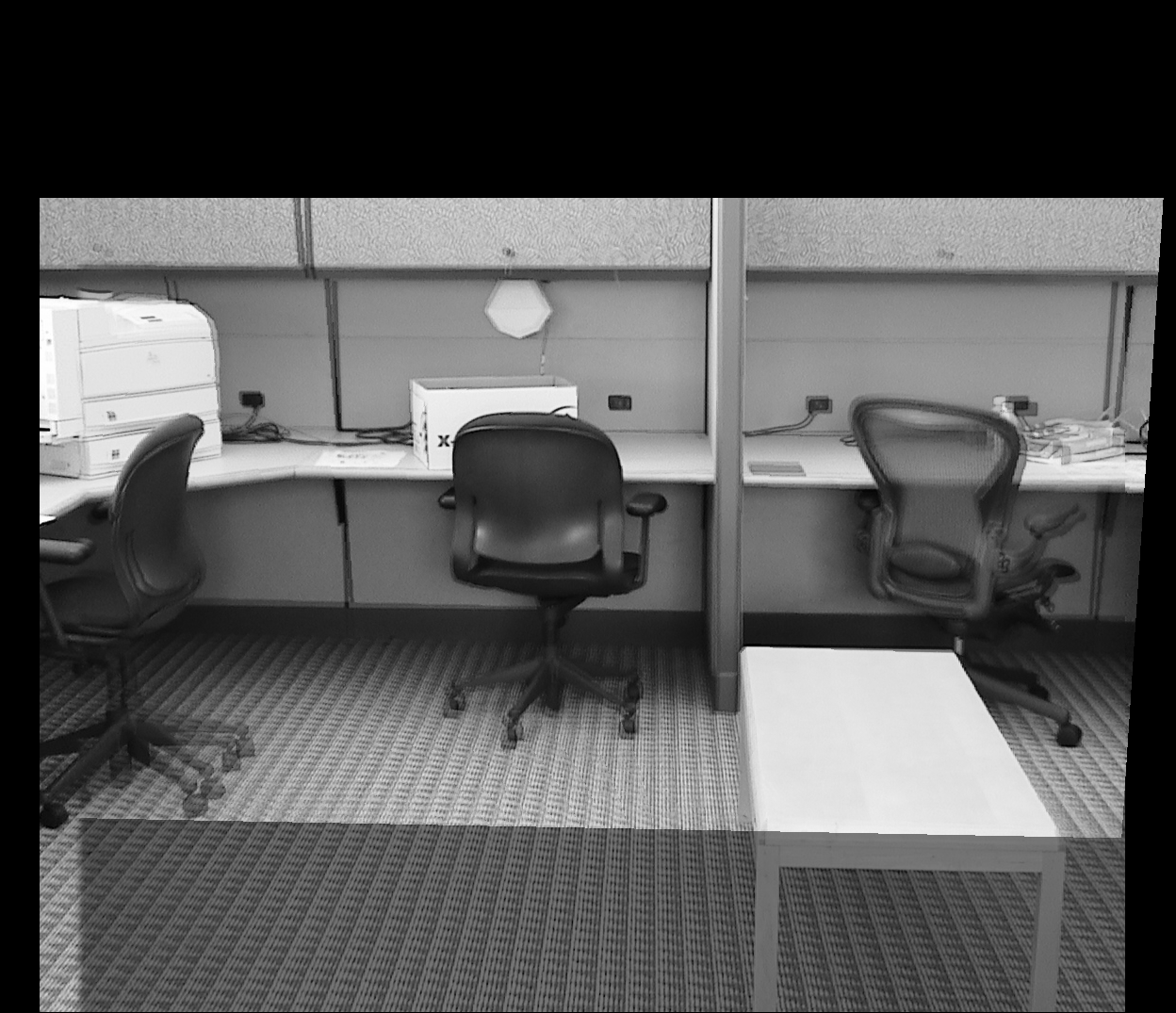
After matching features and getting lists of corresponding points, it is now possible to compute a homography. We do a 4-point RANSAC, by sampling 4 correspondences at random, and computing a homography. Once we have the homography, we warp the second image's feature points and calculate their distance to their correspondence. Any correspondence with a distance within a certain range is considerend an "inlier" and saved to a list. This sequence of selecting 4 points, generating a hommography, and checking distances is repeated many times, and the longest list of inliers is kept.
|
|
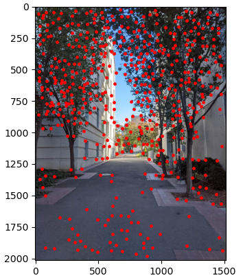
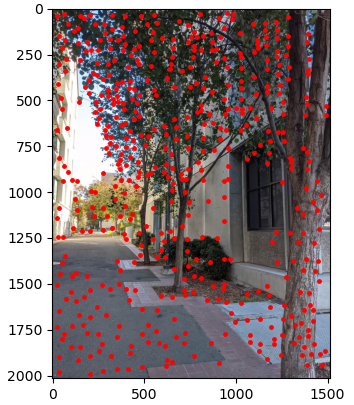
RANSAC'd correspondences
We then create a new homography with the saved inliers, and use this to warp/blend the images the same way as in Part A.
|
|
|
Blended Images
Before this project, I never though much about how panoramic photos were taken. Previously, I thought it had to do with "recording" the movement of the camera, kind of like unrolling a roll of tape from curved to flat. This project has allowed me to understand how panoramic pictures are several photos transformed and stitched together, and how some linear algebra and other creative application of math can change the point of view of a camera and drastically alter perspective.