The fifth project involved warping, stitching, and blending a series of images from the same view point to create a panorama photo.
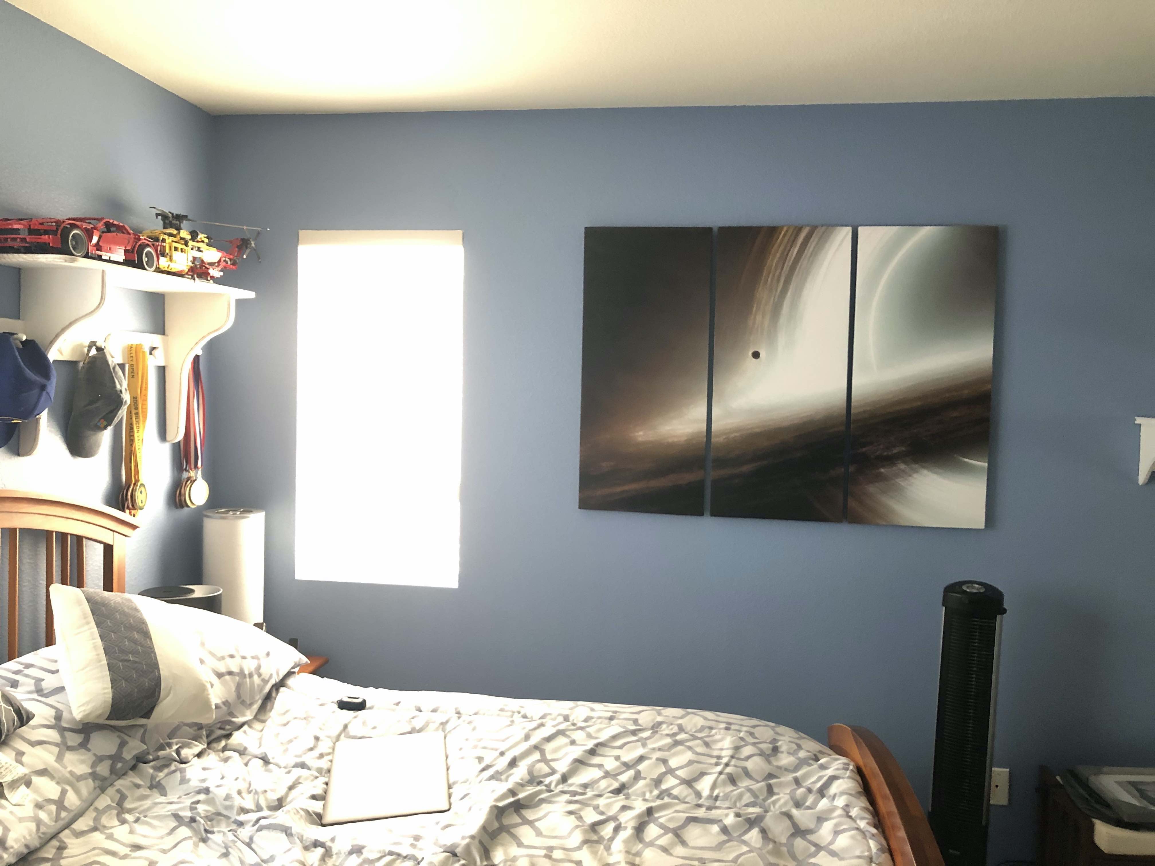
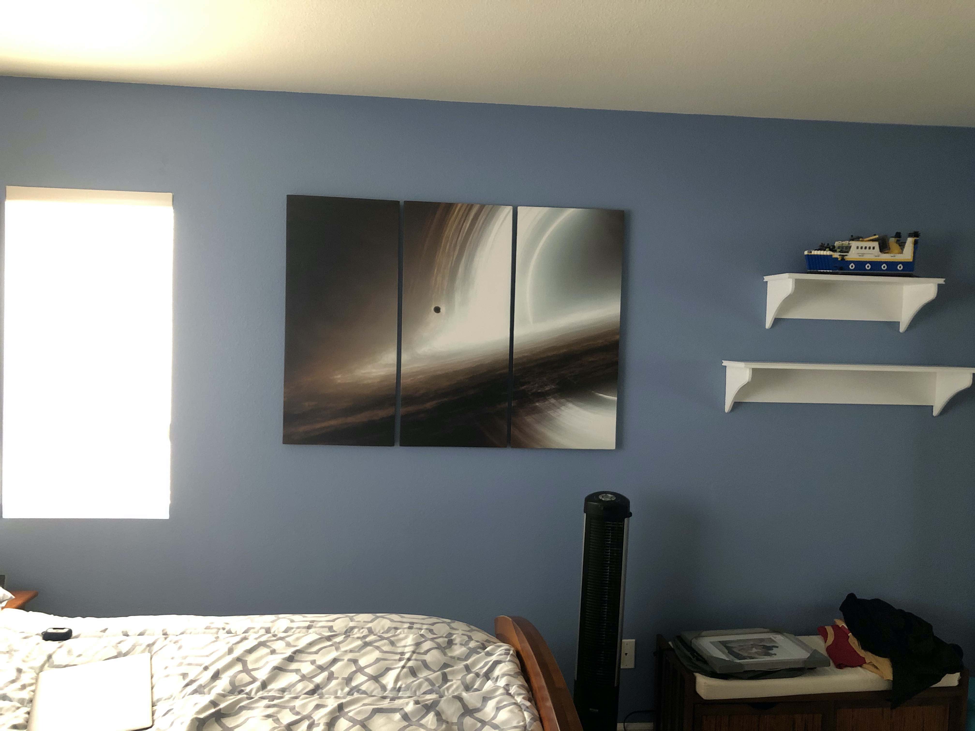
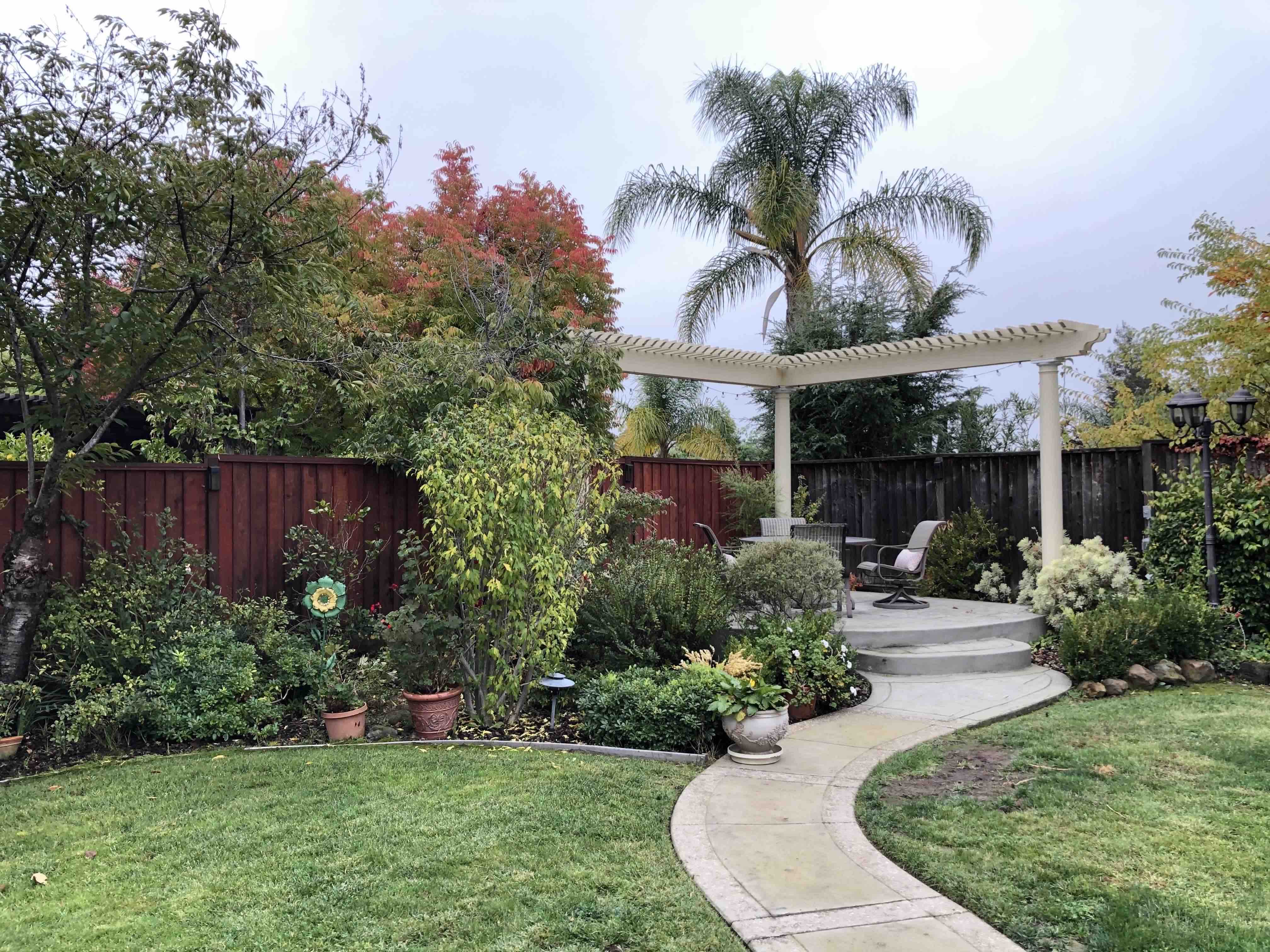
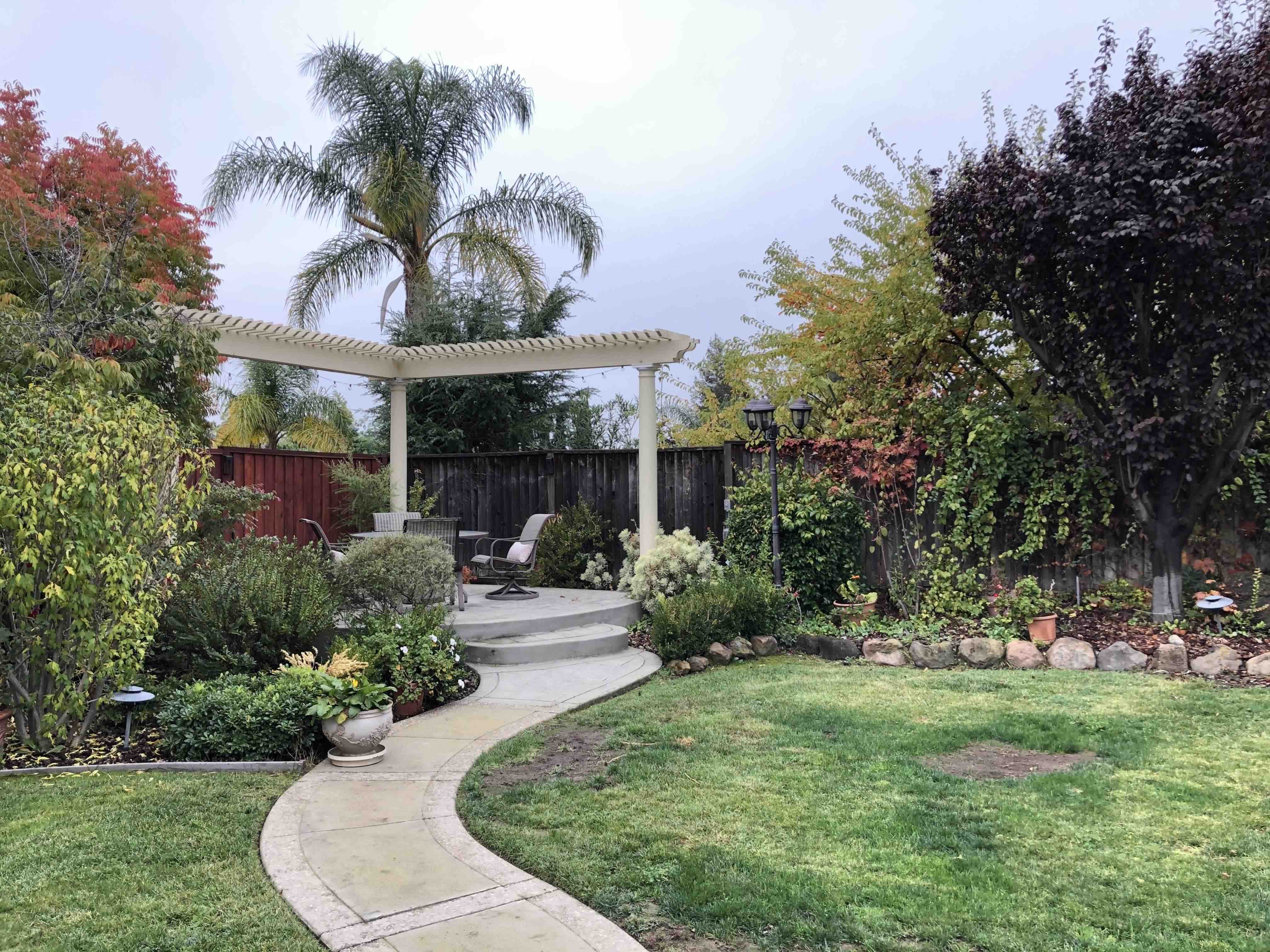
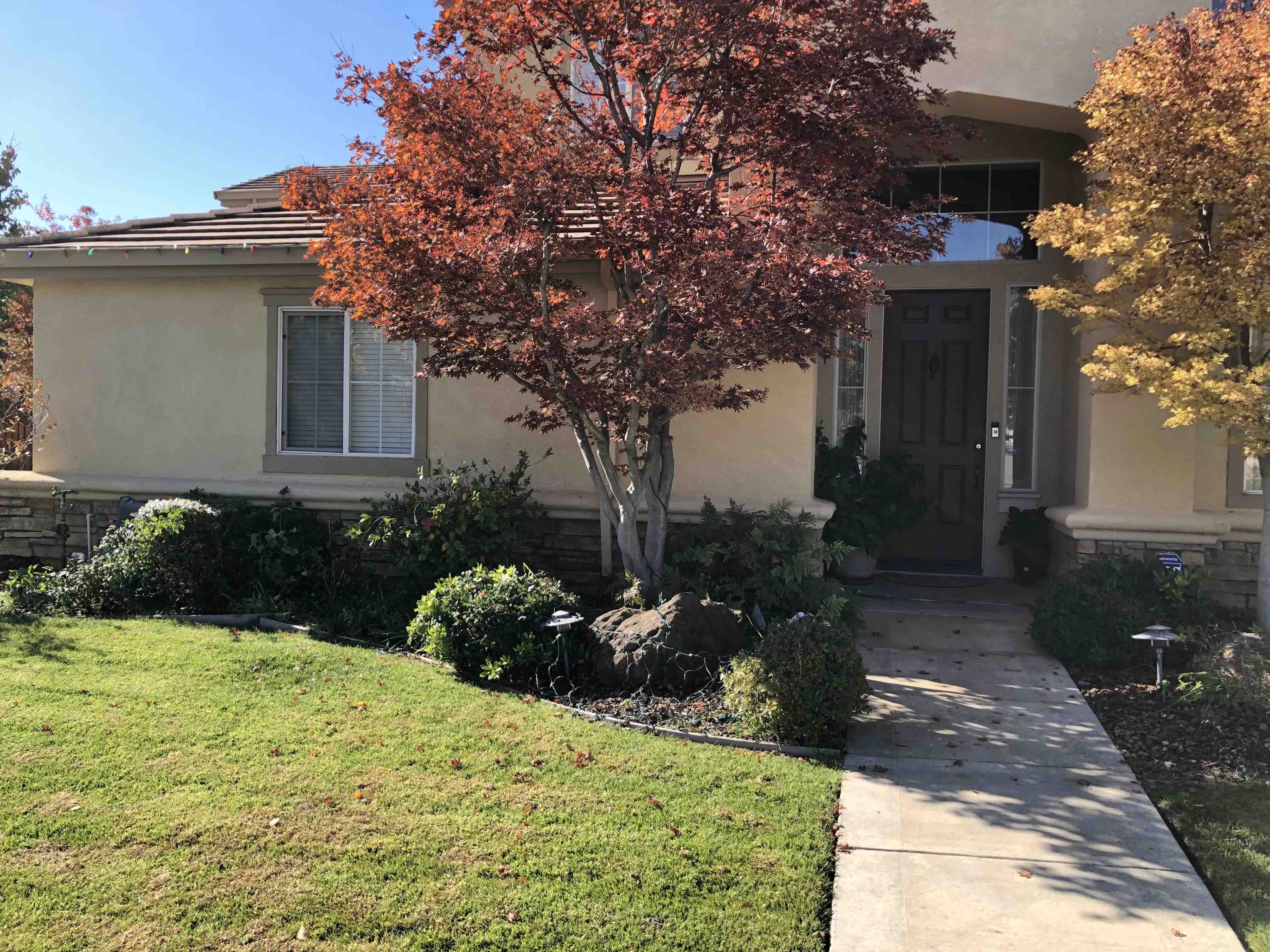
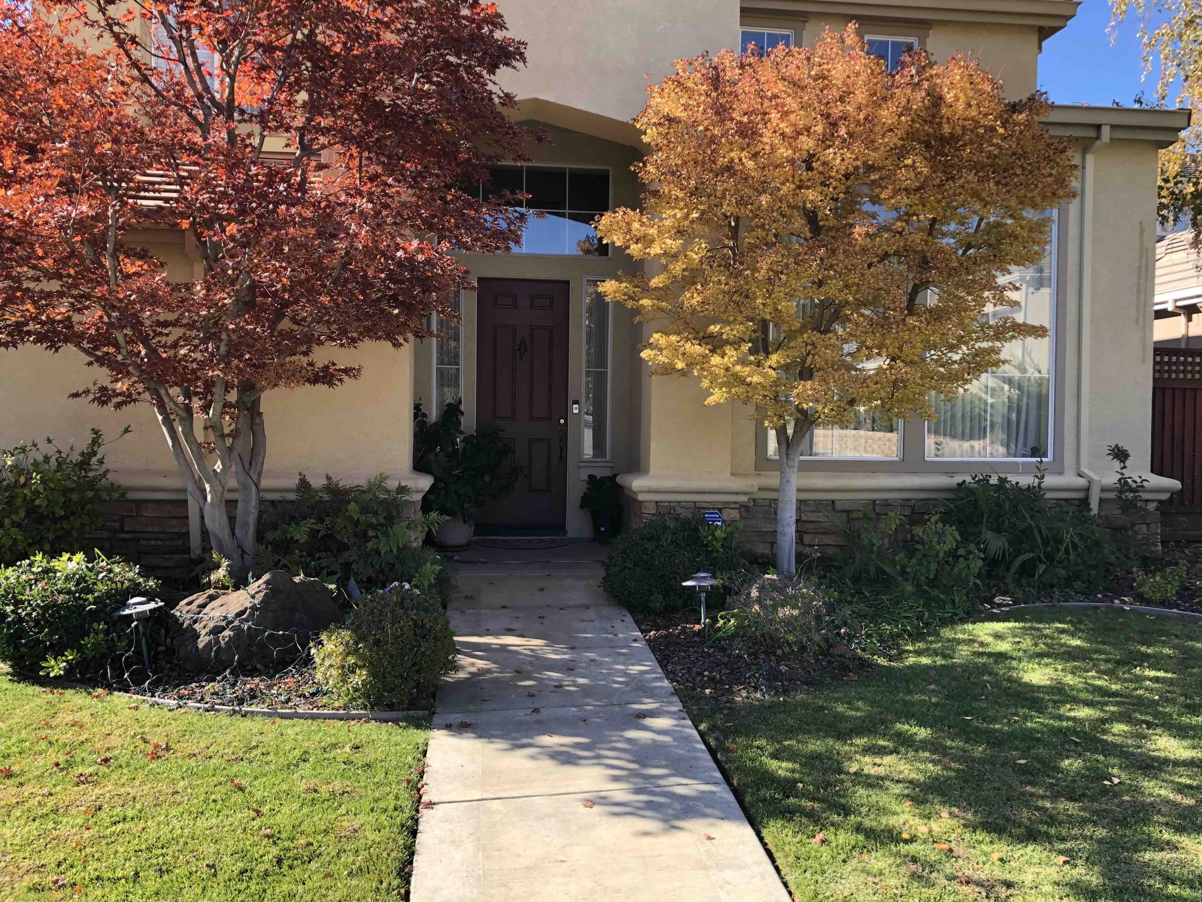
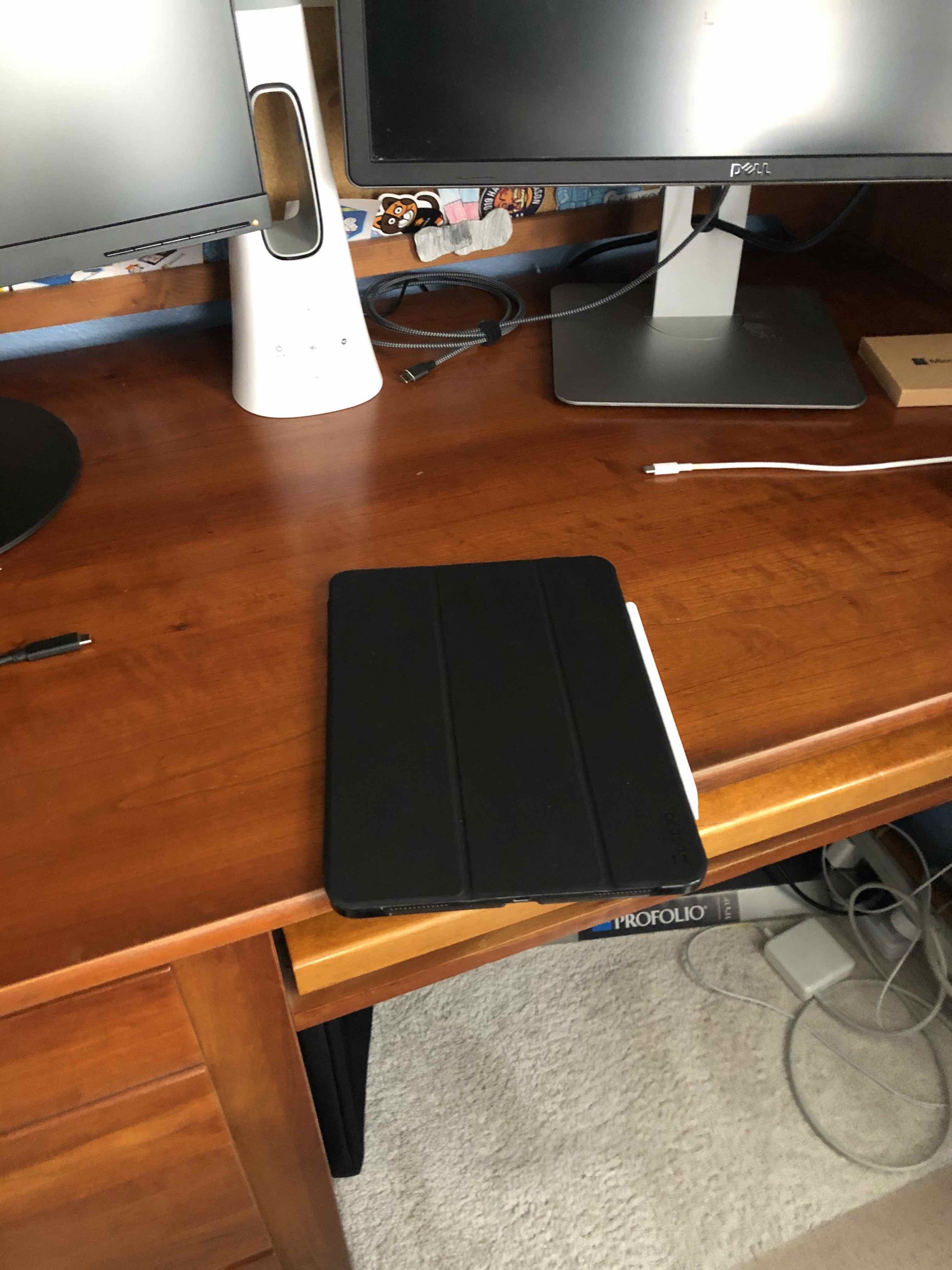
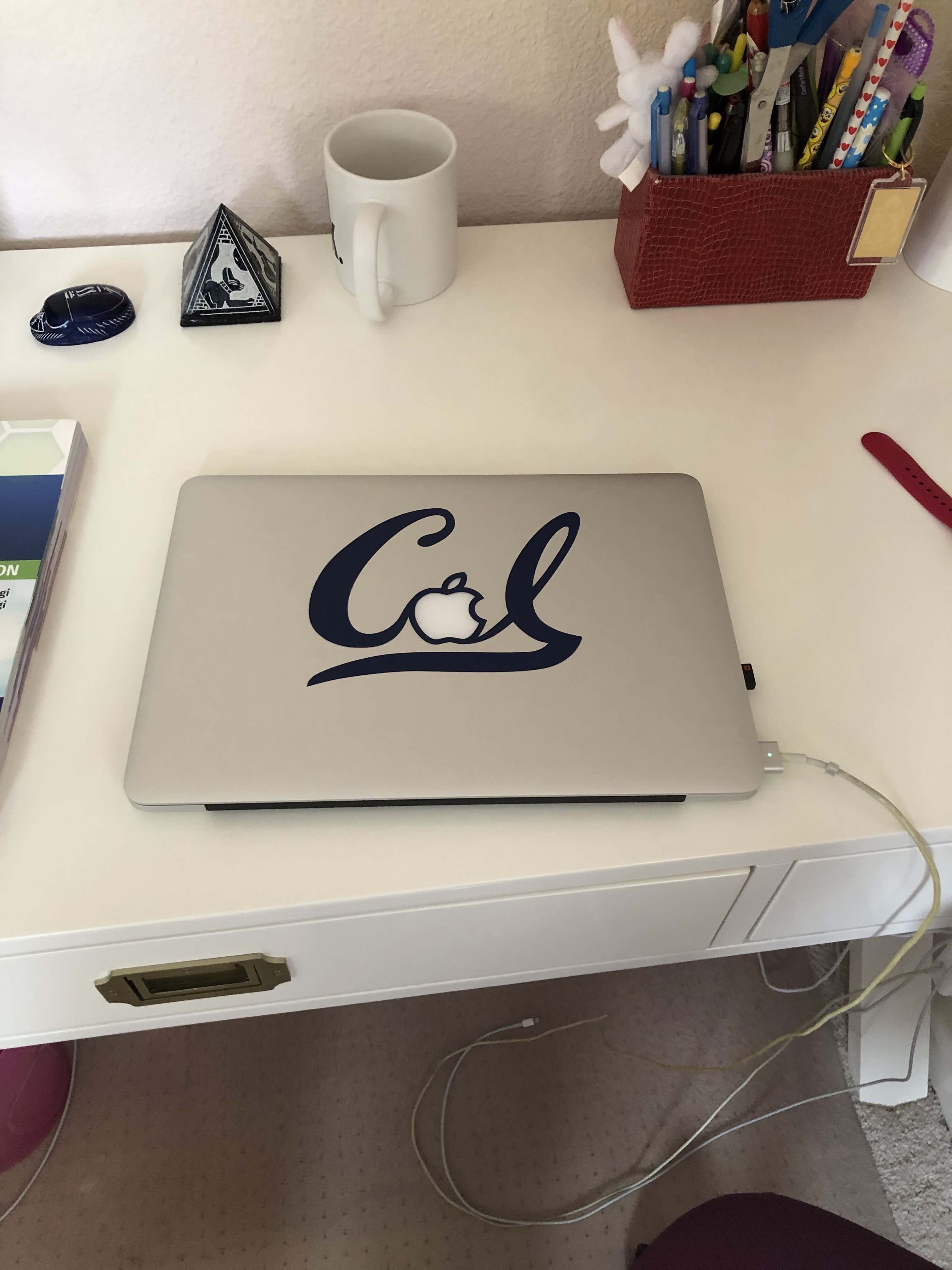
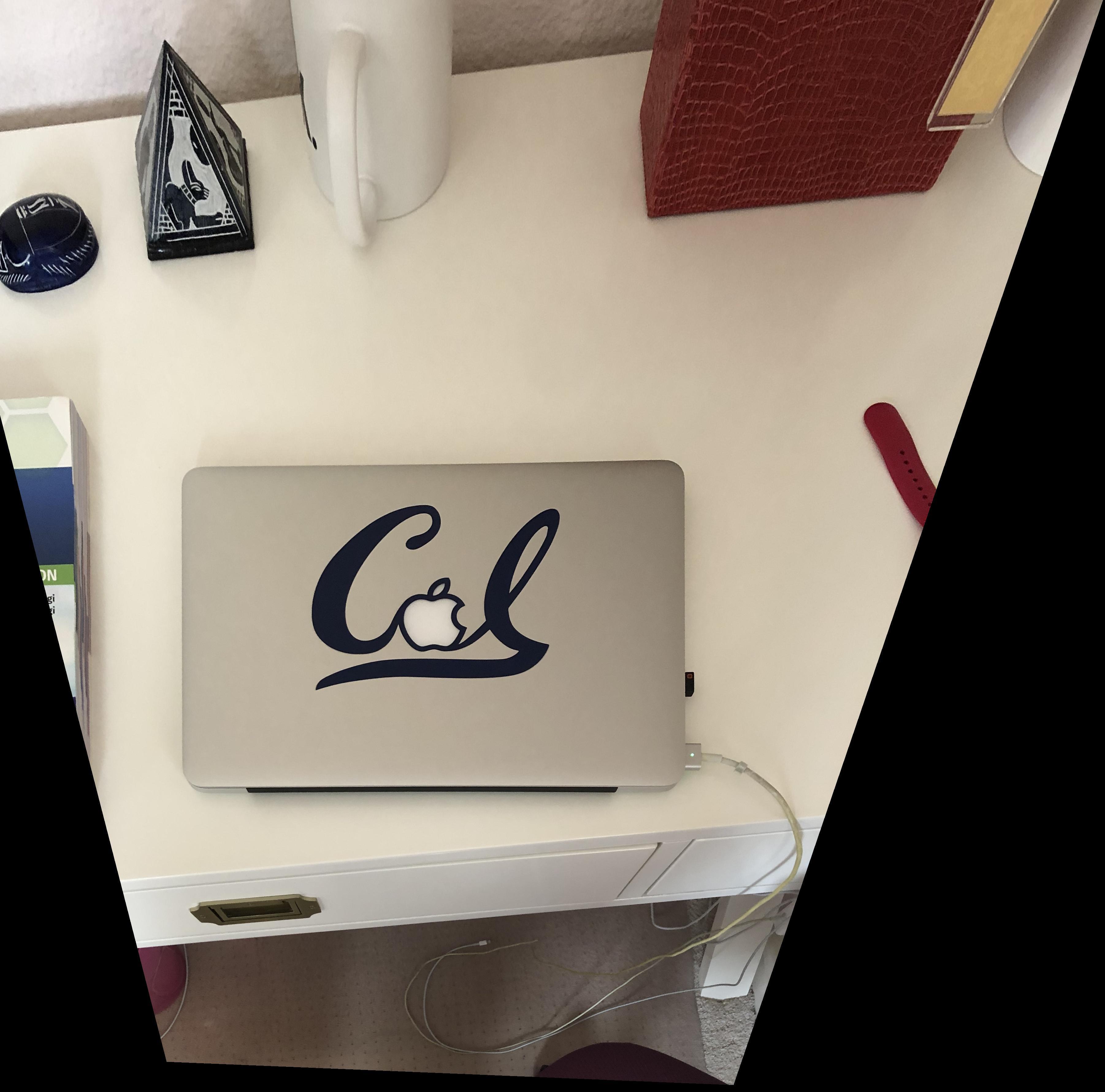
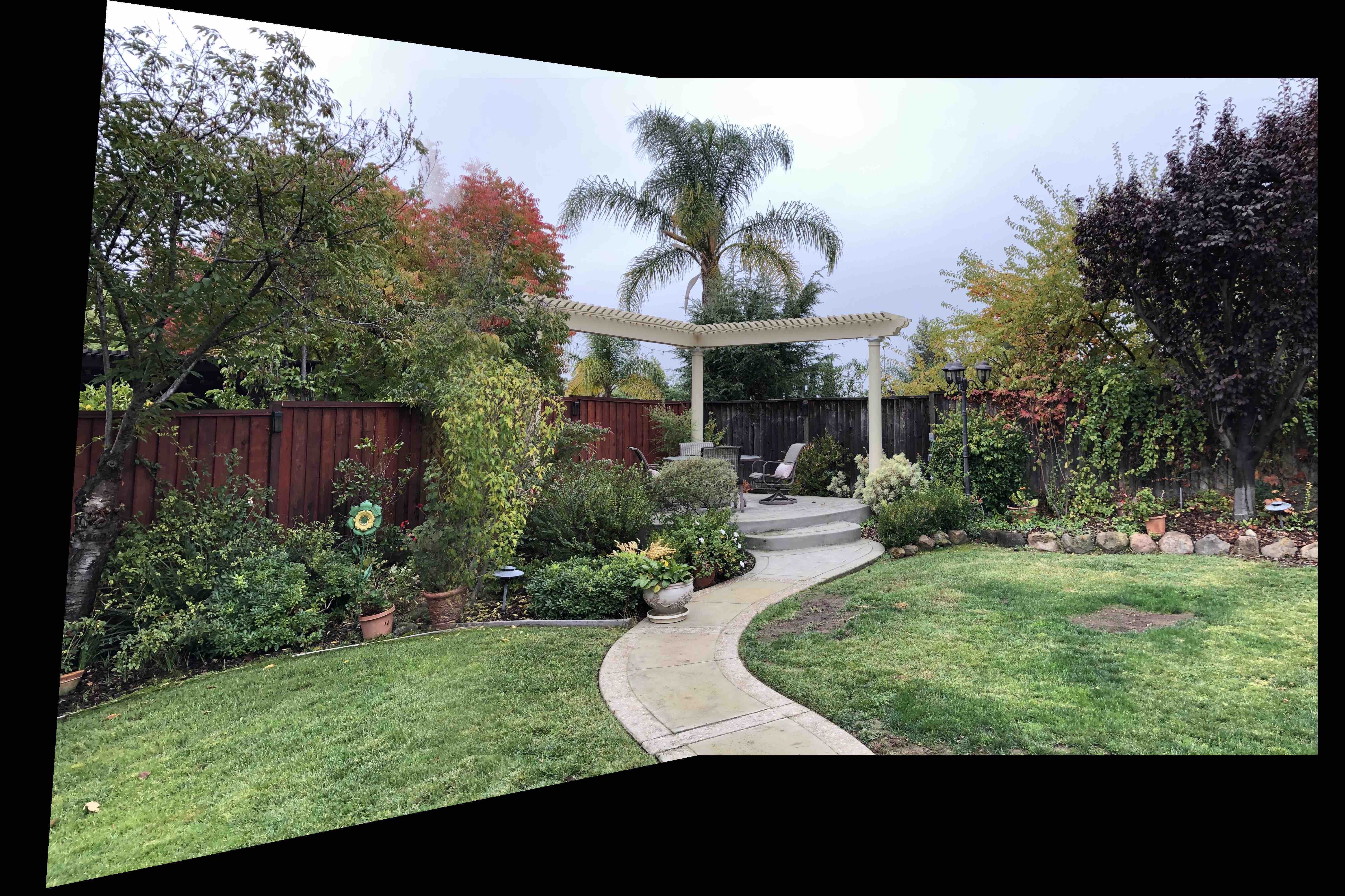
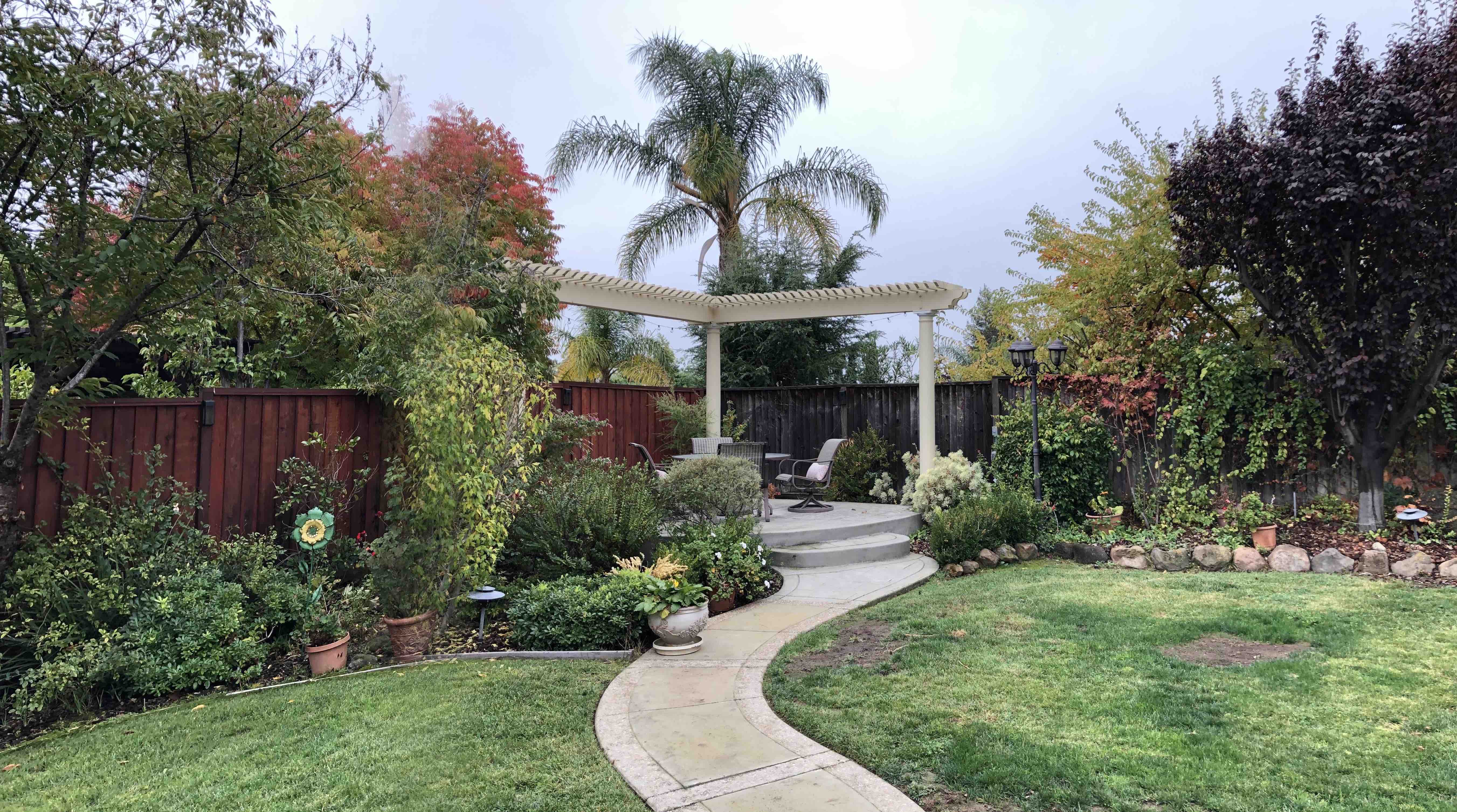
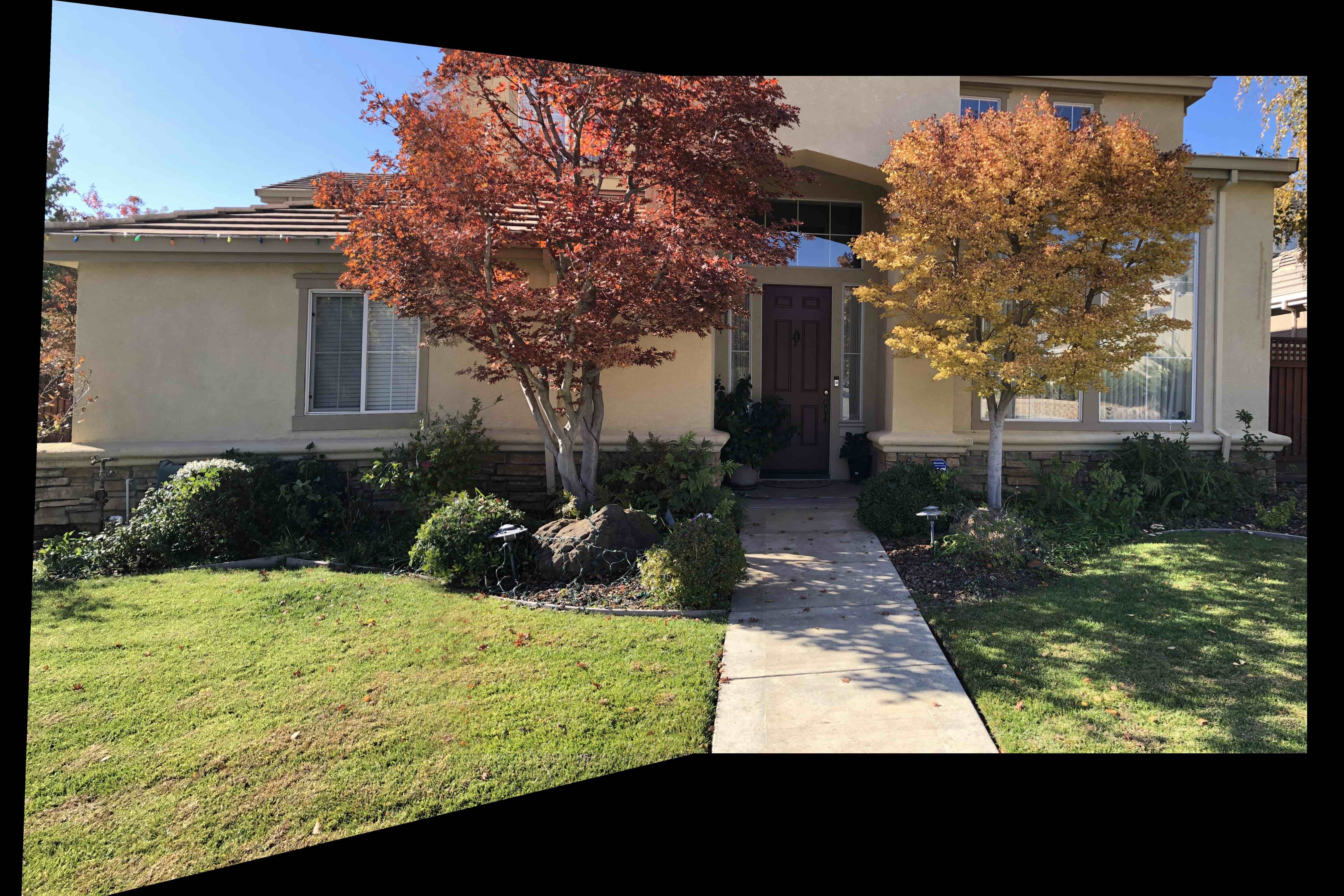
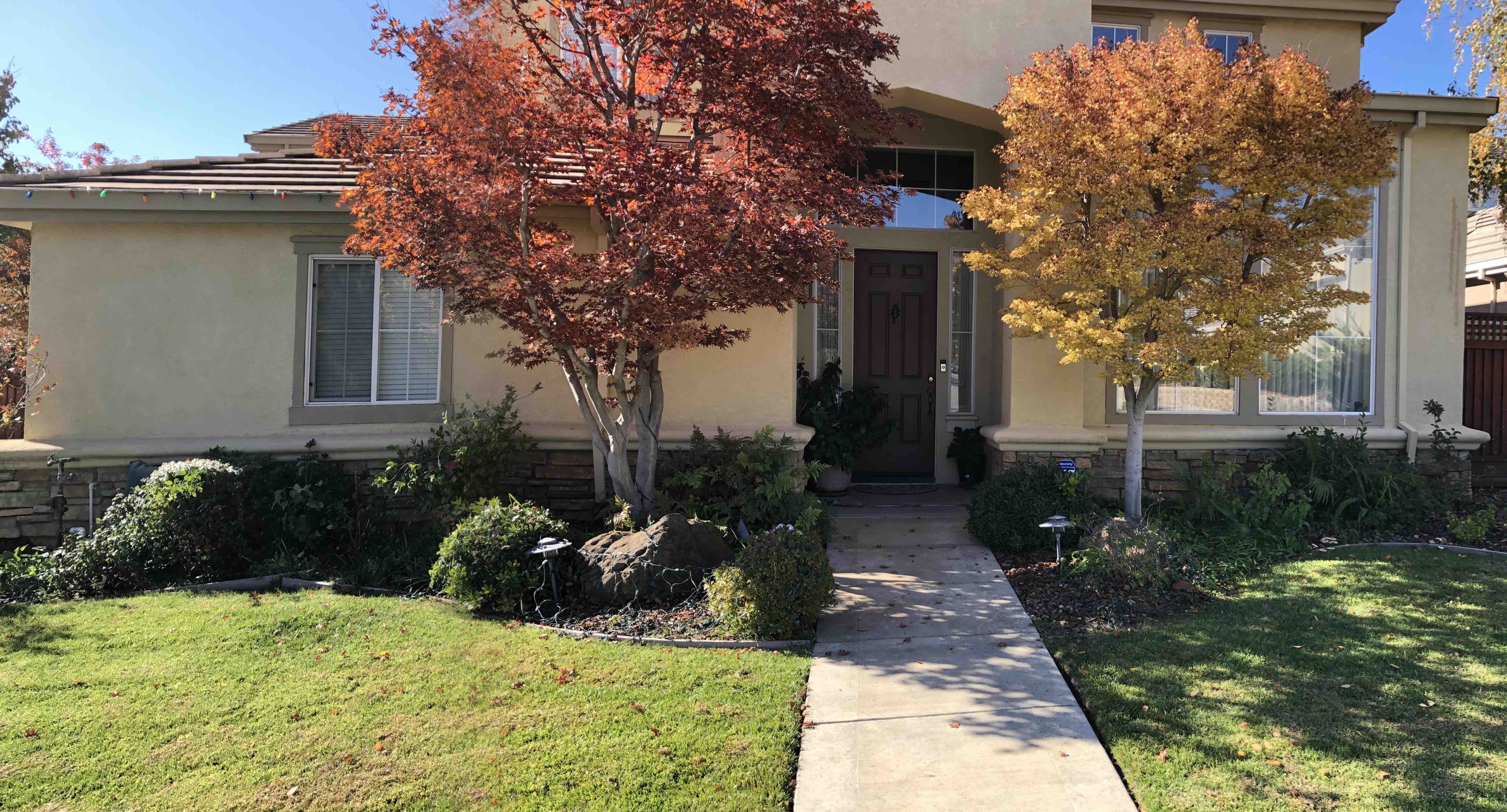
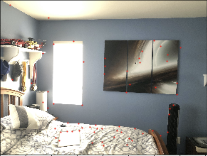
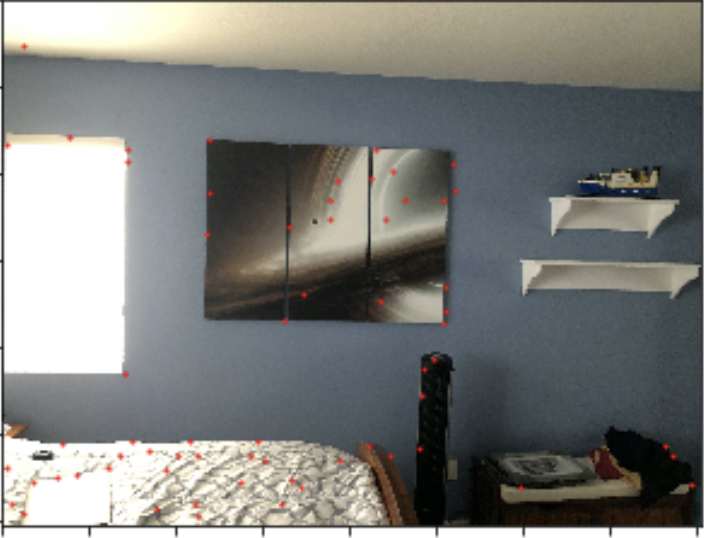
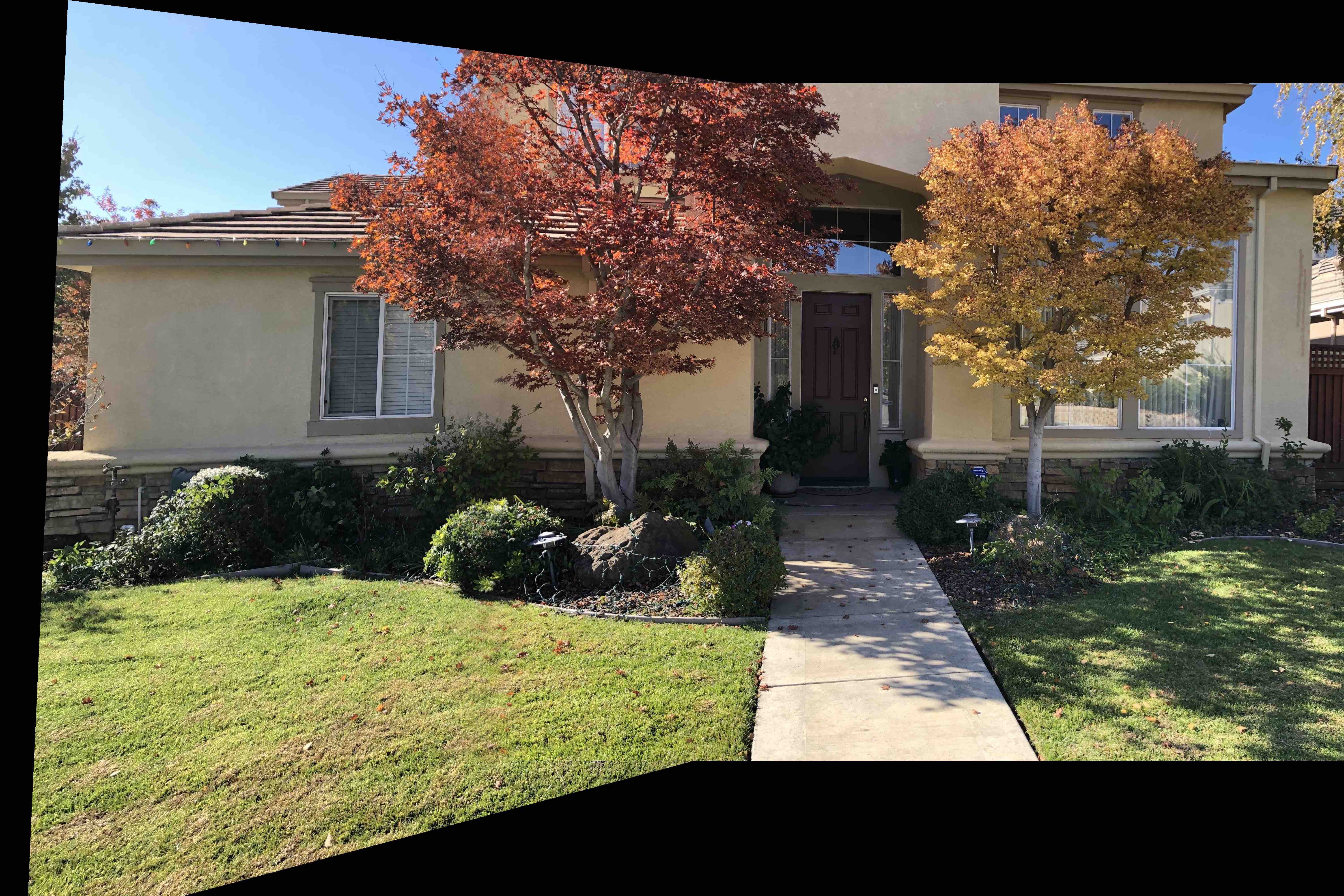
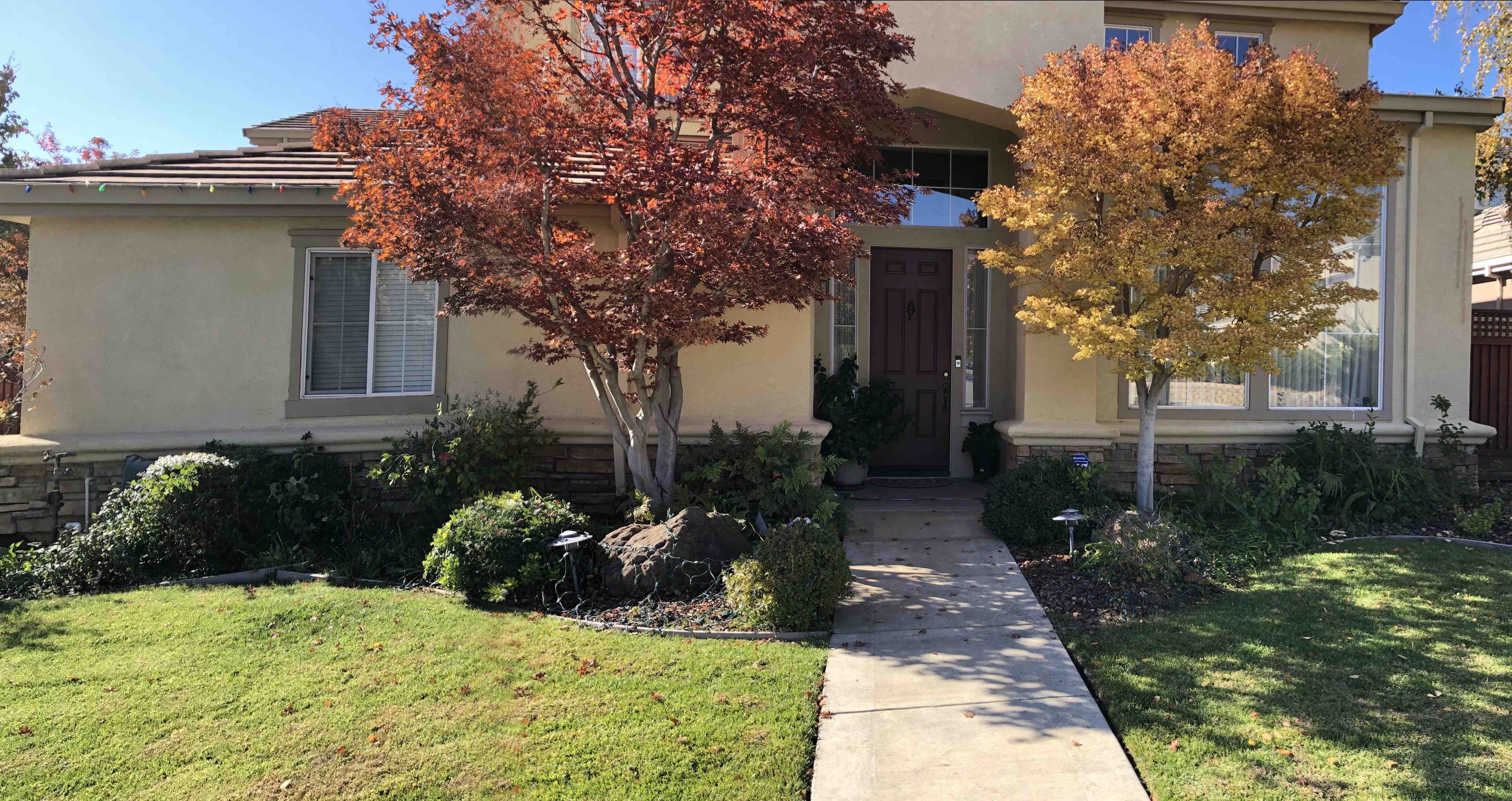
For the first part, I went out and took some photos around my house. In order to take a good set of photos that would create seemless mosaics, I picked a single spot to stand. I captured the desired scenery by taking 2 photos with around 70% overlap between each photo. I used AE/AF lock and only rotated my camera from a stationary position. Here are the photos I took:
In order to recover the homography, I defined a set of correspondences between the images using a simple ginput tool. I reshaped the correspondences to match a least squares problem of the form A * h = b. Here is the exact form of the problem:

I then reshaped the h vector to be 3x3 and then calculated a simple translation matrix to add to h which would allow for the warped image to span the entire output image since certain mapped coordinates would be negative.
Using the newly calculated homography matrix, I first calculate a bound box which will completely define the output warped image. Using this, I extract a list of coordinates that encompass the polygon bounded by these 4 coordinates. I then use inverse warping and interpolation to determine the values of these coordinates of the warped polygon.
Here are a few sample images of the warping procedure converting nonplanar view to planar view of an object identified in the photo:
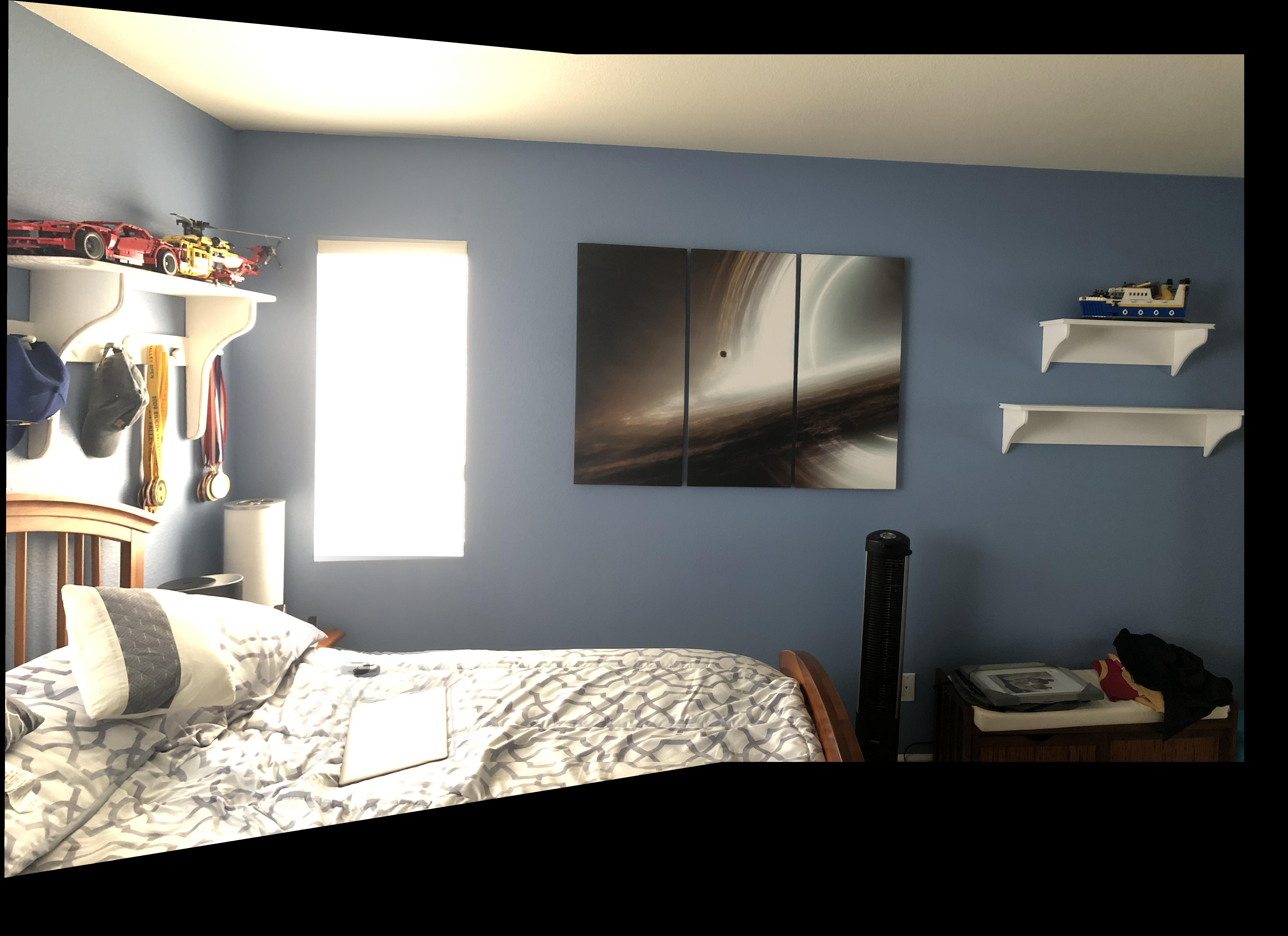
Now that I can succesfully warp images, I used the previous photos I shot and developed mosaics. I annotated 10-12 correspondence points between the images and then calculated the homography matrix. Then, I used the warping subroutine to warp the left image to the right image. I translated the unwarped right image to overlap the warped image at the defined correspondence points. In order to blend the images, I used pixel weighted average. I essentially defined a fractional area of the unwarped image which determined the distance from the seam edge to blend. Then I generated a linear step up matrix that determined the weights. I then overlapped the images by multiplying by this weight matrix. This worked pretty well. In certain areas, it left a slight ghost effect but it's very hard to notice.
Overall, this project was very interesting because I learned how a device like a smartphone is able to generate panoramic photos (although right now I manually annotate). I learned how to generate homography matrices and how to overlap and blend images smoothly. The coolest thing was warping the images and seeing it almost magically line up with the unwarped image.
For the second half of the project, we had to implement algorithms to automatically annotate each input image with correspondences. Then, we could leverage the mosaic creation from the first part to generate automatic mosaics.
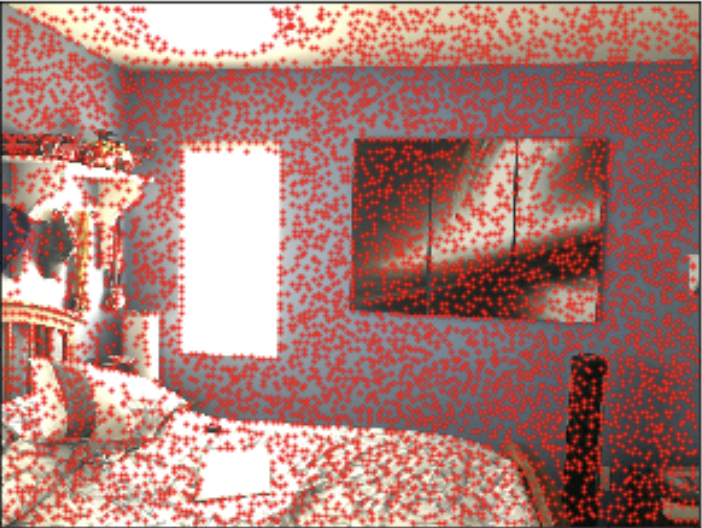
I started by generating annotation points for the input images. These points of interest are corner points across the images. We can use the Harris Interest Point Detector to find these corner points
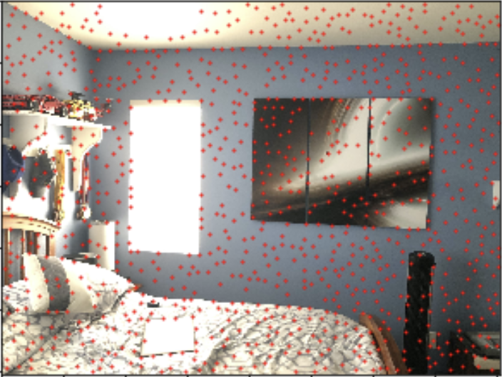
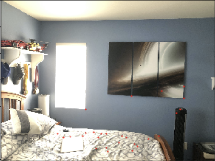
Now that we have a lot of interest points, we need to select a subset of these points to use. We want to pick points that have high Harris values. However, simply selecting the max points will often lead to spatial clumps of points being selected. In order to have a widespread sample which still have high harris values, I implemented Adaptive Non-Maximal Suppression. For ANMS, we essentially want to select the points that have the largest radius to a neighboring point with a higher harris value. For example, the global maxima harris value point will have a radius of infinity since no neighbor is larger. In order to implement, I analyzed every harris point selected, used a K-D tree to create a list of nearest neighbors sorted by distance, and selected the closest neighbor that had a higher harris value. The distance of this selected neighbor is the radius which we will record for the point of interest. After calculating the radius for all points, I sorted the radius in descending order and selected a subset of the points with highest radius.
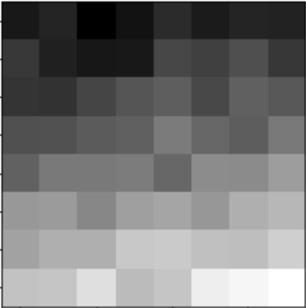
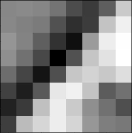
Now that we have a more manageable set of points in both our input images, we now need to uniquely identify each point by its surroundings so it can be matched later. I took each interest point and created a 40x40 patch around. I downsampled to create an 8x8 patch, normalized this patch, and shaped into a vector.
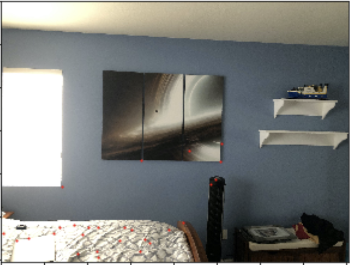
Now that we have all the feature decriptors, we can now find correspondences between the 2 images. In order to do this, I employed a hybrid method which involved Lowe's method. I once again used a K-D Tree in order to keep track of nearest neighbors and distances. In order to make sure we had one-to-one correspondences, for each feature patch in the left, I would find the closest neighbor patch in the right and vice versa. I would only select the correspondences whose nearest neighbors were symmetrical. Then, I used Lowe's algorithm to further narrow down the valid correspondences to those whose nn1/nn2 ratio was low.
The final step is to select the largest inlier set that adheres to a calculated homography. RANSAC returns the final set of correspondences to use. To generate inlier lists, I selected a random subset of correspondences and calculated the homography using least squares. I then used this H matrix to warp all correspondences. I then calculated the error distance and choose the points within a small error threshold to be the inliers. I generated many inlier lists and chose the largest list as the final correspondences.
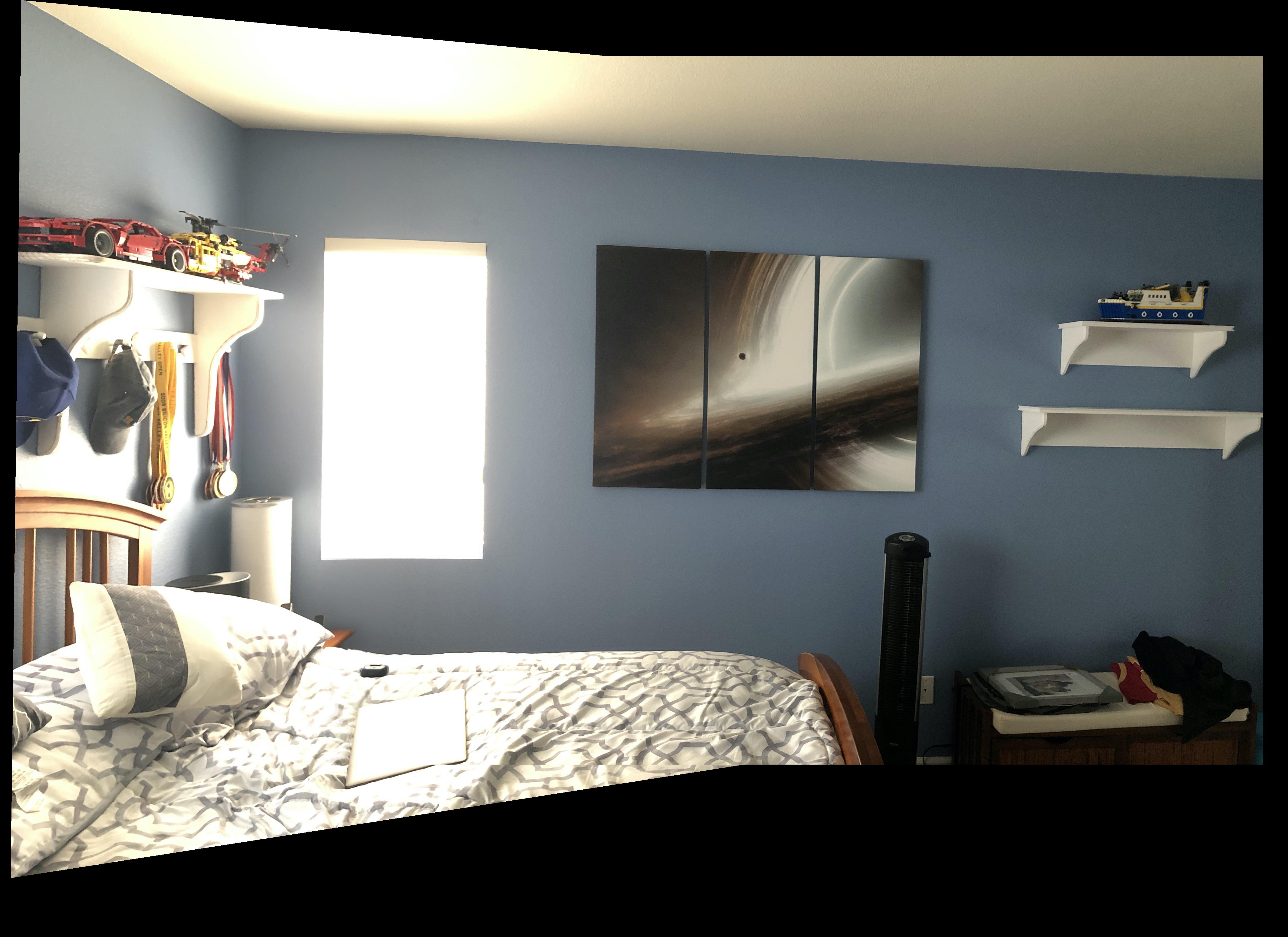
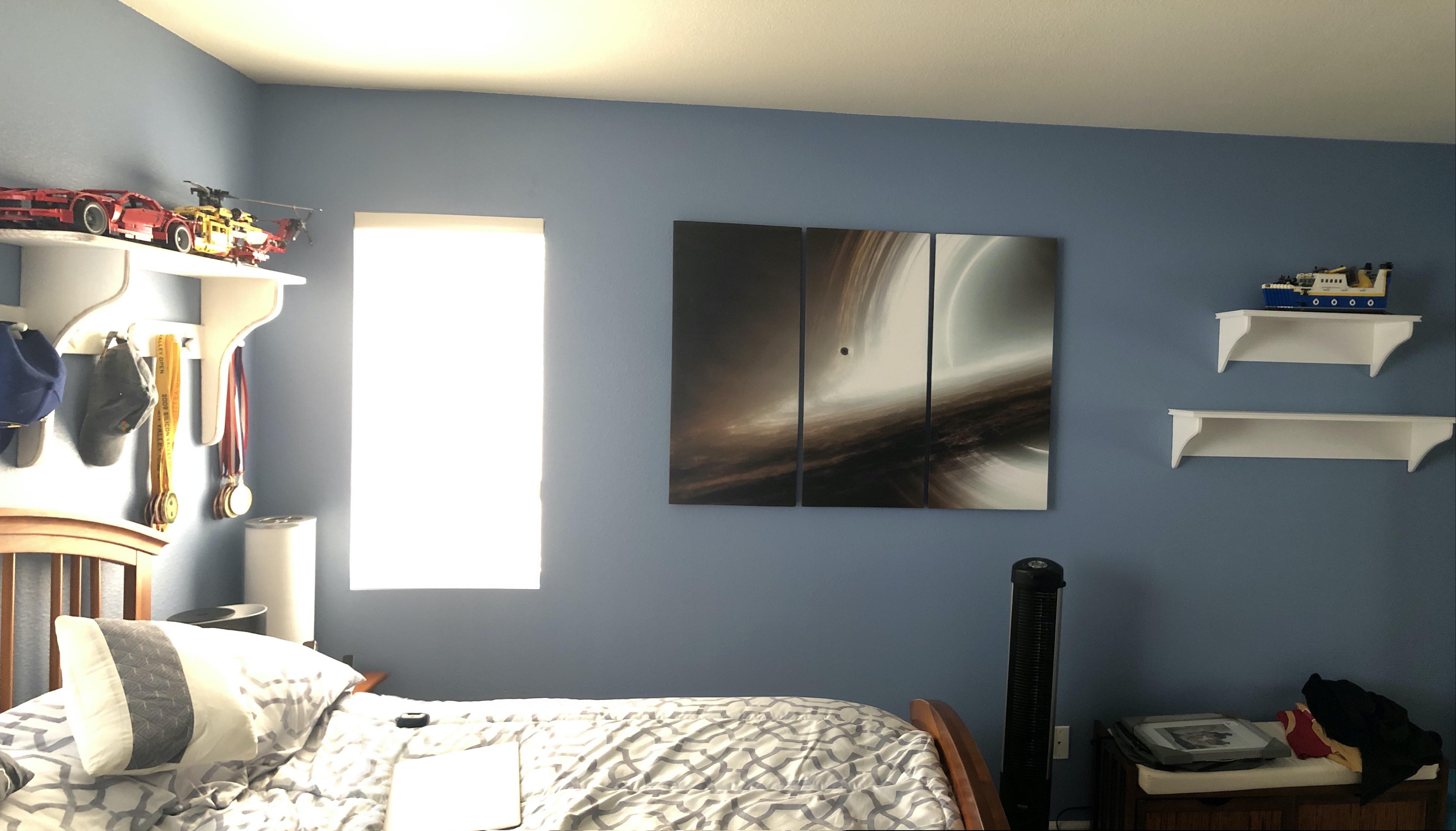
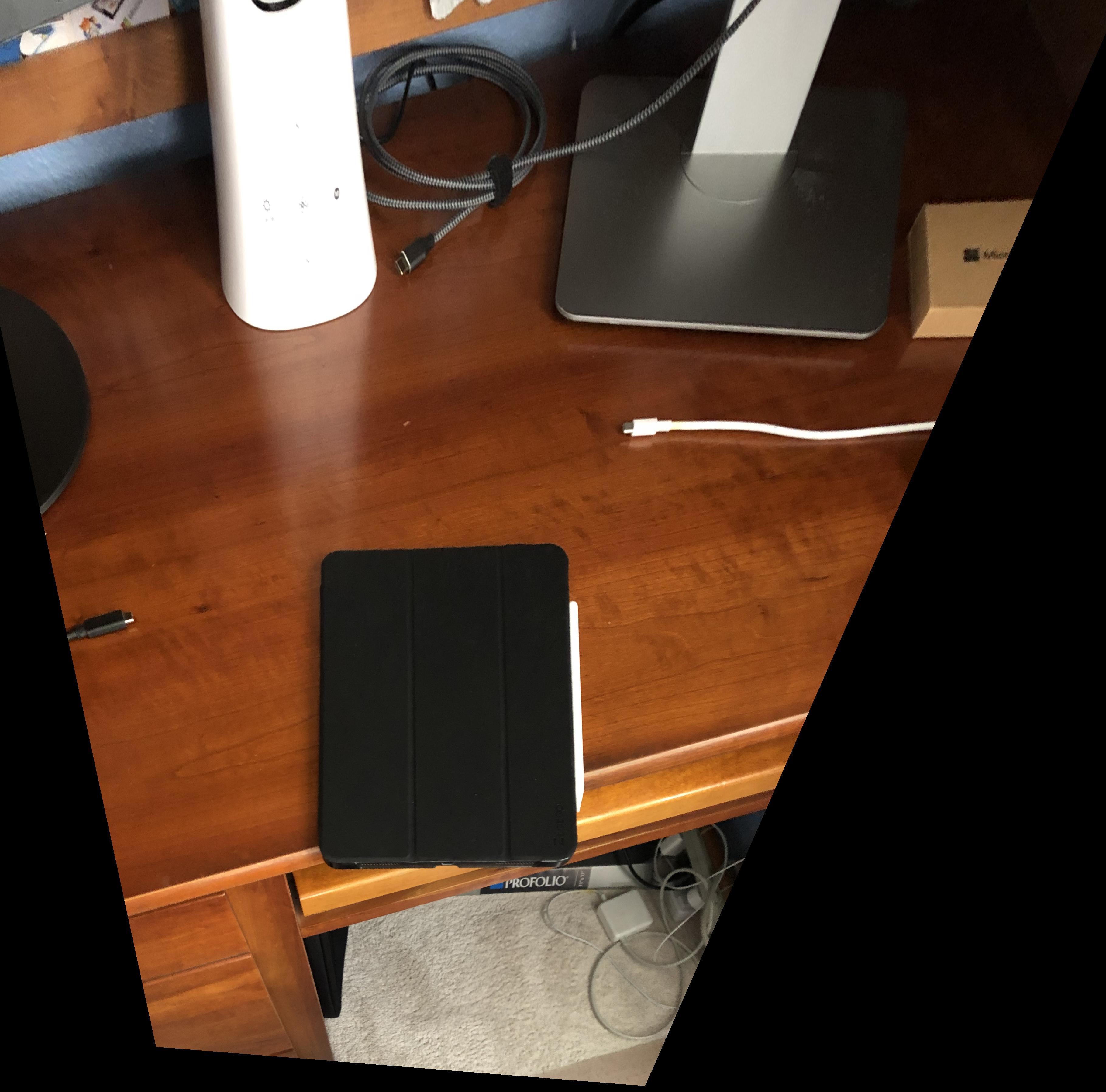
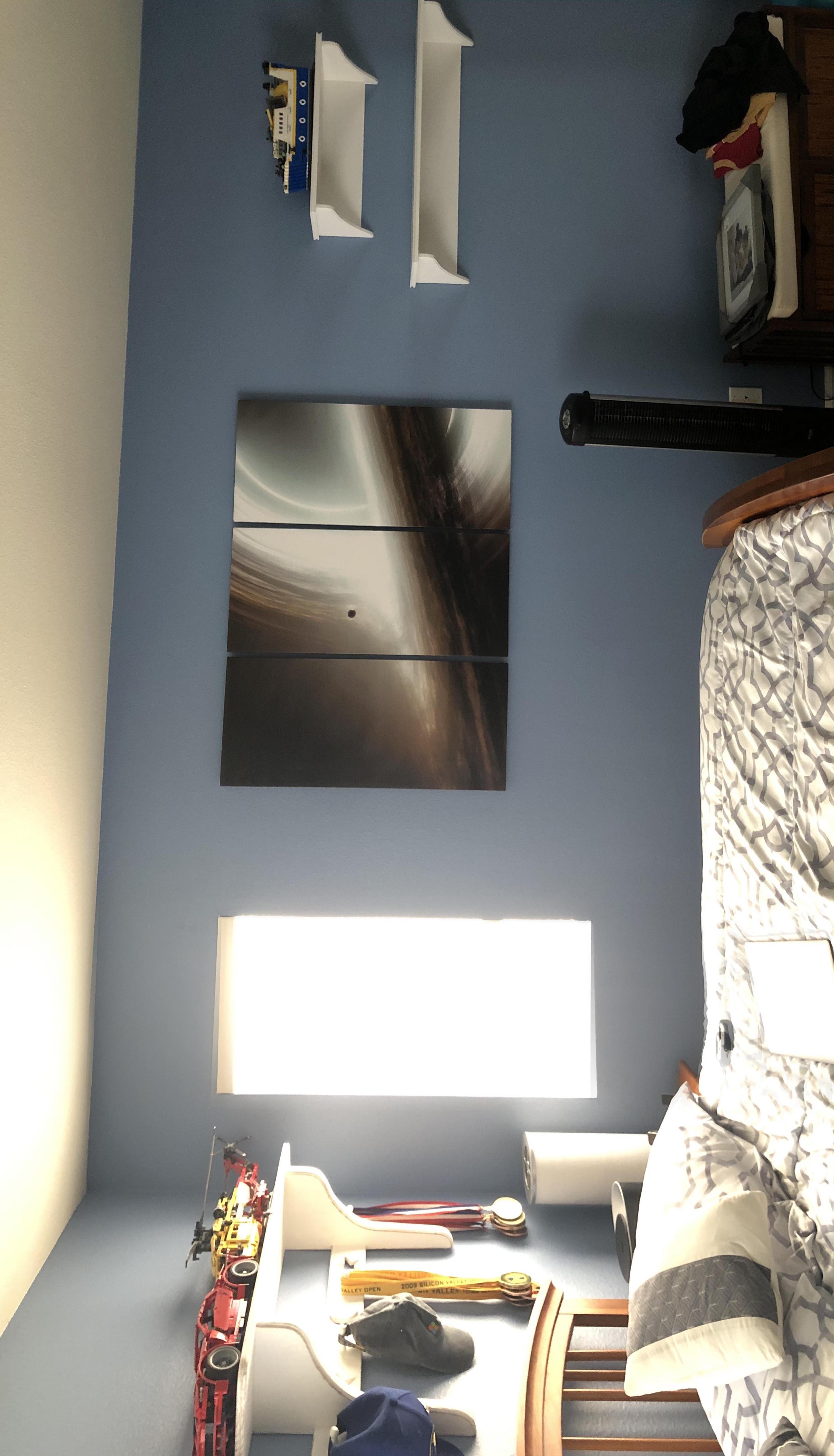
The automatic stitch mosaic is much better than than the manual one. The manual one has ghosting effects around the laptop and window which are caused by the points being slightly off. This is fully corrected in the auto-stitched msoaic.
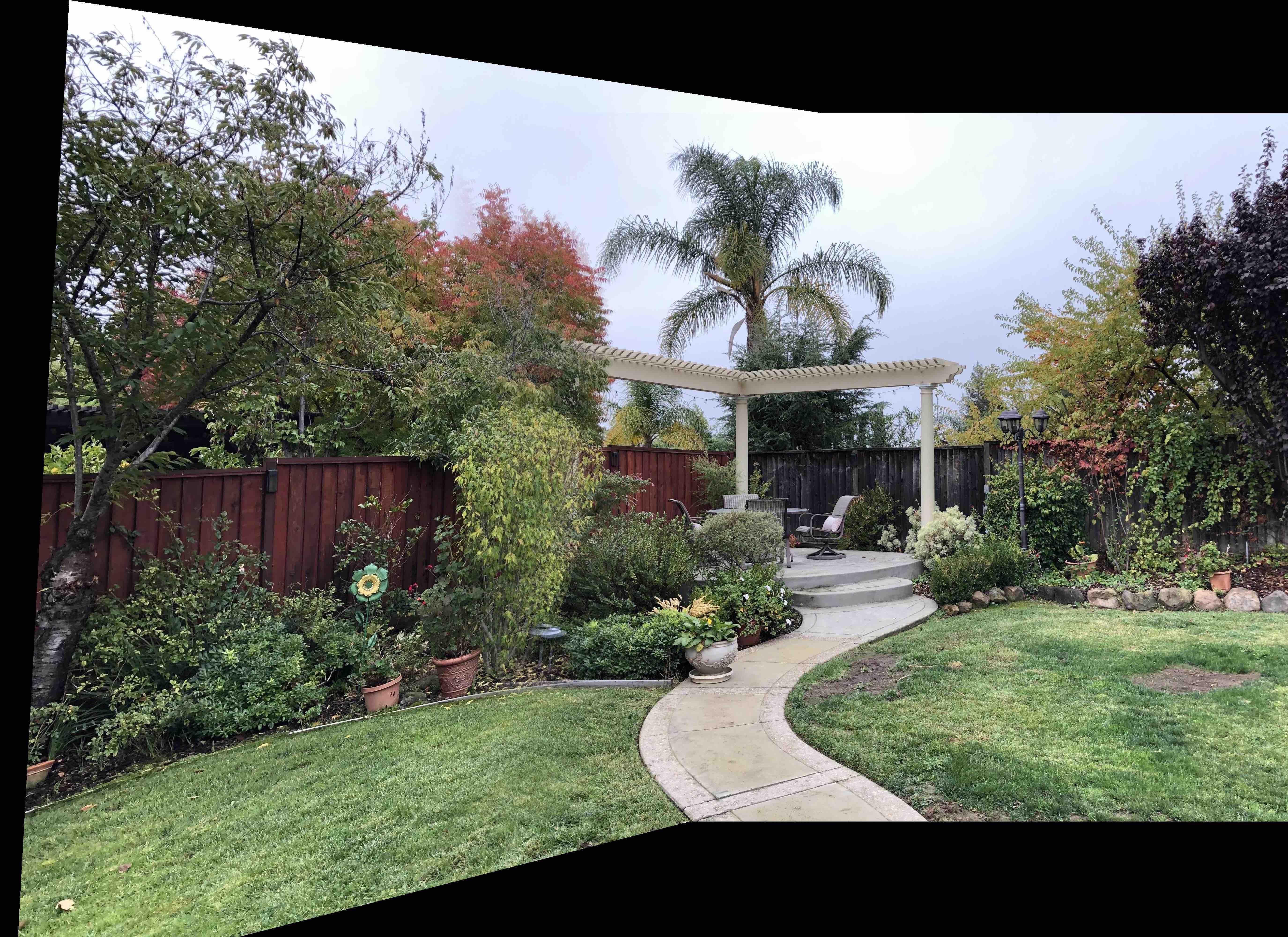
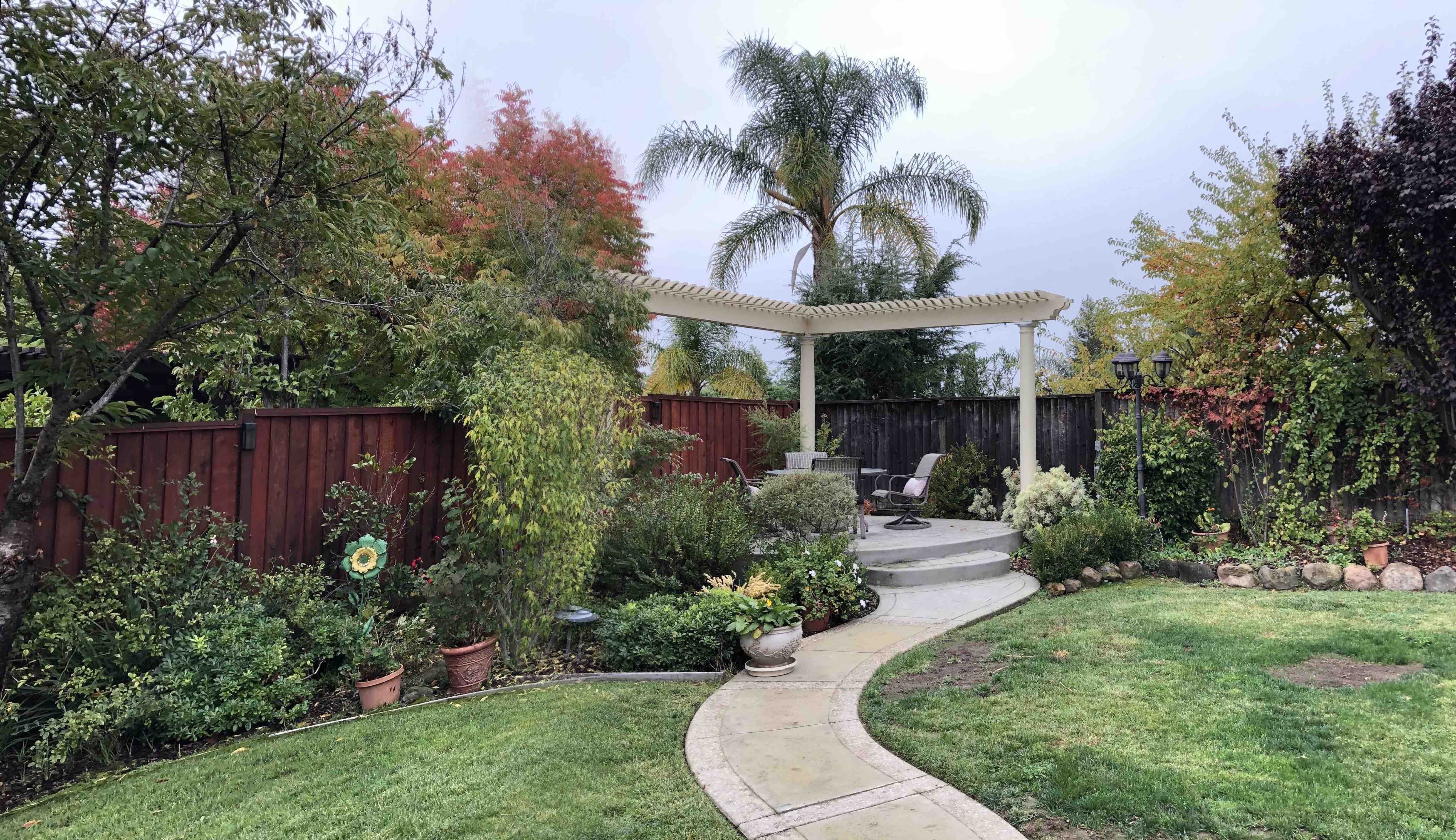
The automatic version is slightly better than the manual. The ghosting around the trees on the left side is much more pronounced in the manual version. The alignment is slighly better with the automatic version and thus ghosting is a bit less. Better blending would also help resolve this issue.
Once again, the automatic version is slightly better. The tree on the left has slight ghosting on the leaves if you zoom in on the manual version. This is corrected in the automatic one.
Overall I learned not only all the calculations and computation required to seemlessly and automatically stitch images together, but I also learned how to efficiently process large matrices. The coolest part was seeing the various suppressive algorithms slowly refine the correspondences until it reached the best set.