Image Warping and Mosaicing
by Pauline Hidalgo
Part A
In the first part of this project, I manually define correspondence points to compute homographies, do image rectification, and create image mosaics.
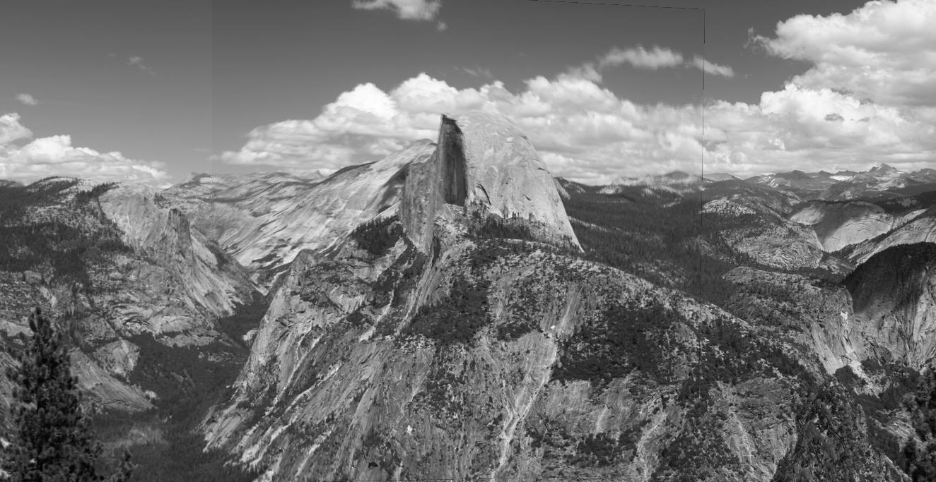
Images and recovering homographies
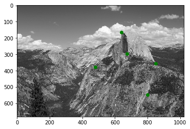
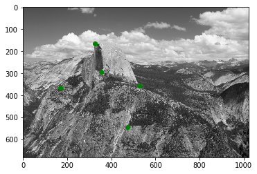
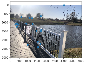
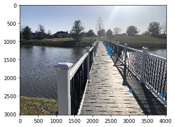
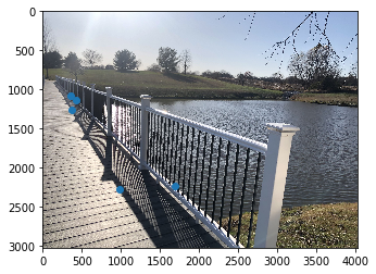
Below are some images I am using to create image mosaics, along with their correspondence points. I found the images of Half Dome online
here. I also took images using my phone, trying to rotate the camera without changing position, and keeping a good amount of overlap. I couldn't really control the exposure settings that well, so some seams are quite noticeable.
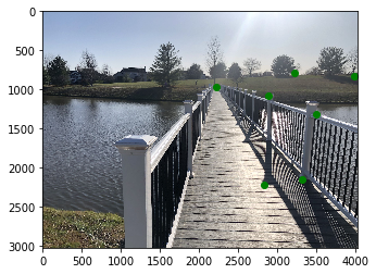
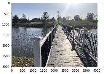
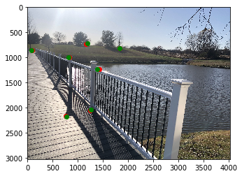
As described in the spec, 4 correspondence points are enough to solve for the coefficients of the homography, but I use more points to improve the accuracy of the homography and solve for it using least squares. I used Photoshop to read off the pixel values and defined the correspondences as accurately as I could, but naturally there are errors. The bridge pictures below show the actual points in green and the remapped points computed using the homography matrix in red.
Warping and rectification
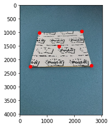
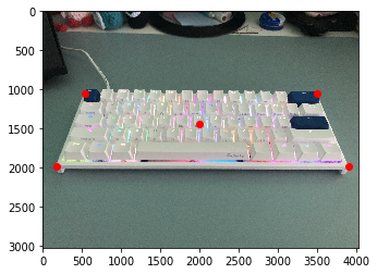
Once H is calculated, I warp the images using inverse warping and interpolation for the pixel values. For rectification, I used my keyboard and a post-it note, which I know should be a rectangle (1:3 ratio) and square from the frontal-parallel perspective.
Image mosaic and blending
From the previous 2 parts, we can now make an image mosiac! One problem I faced was points that were not in the overlapping area of the images got cut off by the warp since they were mapped to negative locations. I resolved this issue by first multiplying the homography matrix by a translation matrix to shift any negative pixel mappings to positive so that they show up in the new image. I also padded the images by the amount of shift to ensure that there was enough space for both images once they are put together. I determined the amount of shift needed to fit both images by eye, which ended up being 4000 pixels for the below images.

left image

right image
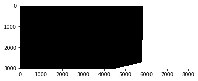
mask
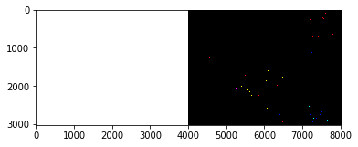
mask
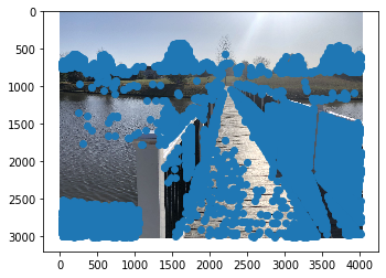
For blending, I took a weighted average of the pixels in the overlapping region. For the regions that did not overlap, I used the masks above to plug in the correct pixels directly into the final image. Unfortunately, the result below still has prominent seams, as well as blurring in the overlapping region! It's particularly noticeable from the many lines on the bridge, though the landscape in the background looks decent. These problems might be caused by error in my correspondence points, slight changes in my camera location (instead of only rotation) while taking pictures, and/or changes in lighting as I was using my phone. For reference, I also included the bridge images just stacked on top of each other, without any blending. Now, there's no blurring, but the seams are stronger.
Part B
In the second part, I use methods from the paper
"Multi-Image Matching using Multi-Scale Oriented Patches” by Brown et al. such as corner detection, ANMS, nearest neighbors, and RANSAC to automatically define correspondence points and stitch images.
Feature Detection and ANMS
Harris corners for each image were generated using the Harris point detector provided in harris.py.
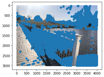
Adaptive non-maximal suppression is used to pick strong corner points and ensure a good spread across each image. Below are the images with all of the harris points and the top 500 points (highest r_i values) from ANMS.
all harris pts

after anms
all harris pts
after anms
Feature Patches and Matching
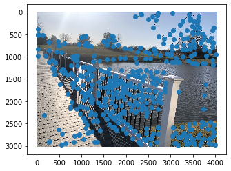
The feature descriptor for each point is a grayscale 40x40 patch centered at the point, blurred for anti-aliasing, then downsampled to an 8x8 patch. This patch is also bias/gain-normalized to account for differences in brightness. Then, using SSD as the distance function, nearest neighbors is used to match points between the two images based on the feature patches. To avoid bad matches, we check that the first nearest neighbor is significantly better than the other options by only matching if 1-NN error / 2-NN error < .3. The threshold of .3 was picked following Figure 6B of the Brown et al. paper.
Below is an example of two patches that were matched, along with all the points that were matched between the two images.

example patch from left
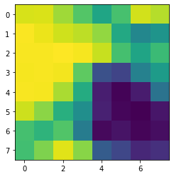
example patch from right
nn left correspondences
nn right correspondences
Outliers
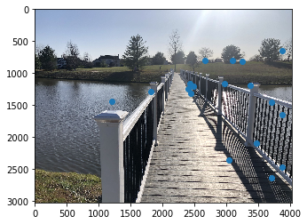
There's some decent matches from above, but there's also quite a few that are off or in non-overlapping areas (on the leftmost railing, tree branches on the far right, etc.). Because least squares is very sensitive to outliers, we additionally do RANSAC on the matches to ensure the correspondence points will create a good homography. In the RANSAC loop, inliers are set to be matches whose dist2 using the computed homography is < .5.
before RANSAC
before RANSAC
after (final points used)
after (final points used)
Results
After RANSAC, we finally have a set of correspondence points to warp the images and proceed like in Part A. On the left are the mosiacs from manually picking the correspondences, and on the right is the automatic mosaic.
For the bridge image, it has some similar issues that I faced in Part A (blurry in the overlapping region, visible seams). It's likely because I used my phone camera and may have moved its position while rotating. It's cool to see how the lines on the floor of the bridge actually line up in the automatic version, though.
Learnings
The coolest thing I learned from this project is seeing how much you can explore an image just using different homographies! I also learned how important it is to exclude outlier correspondences, as even one can mess up the warp a lot.