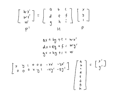
Recover Homographies
ComputeH Method
I used the method below to implement computeH. I stacked all data into matrix to speed up the process.
ComputeH Result


Warp the Images
To warp the images, I built the pipeline below.
1. H @ im to find the shape of target
2. Find the boundary of the mapped points
3. Create the new image base on the boundary
4. Apply H inverse to find the pixel values
5. Filter pixels that mapped to pixels that are out of bounds
6. Assign Pixel values for the new image
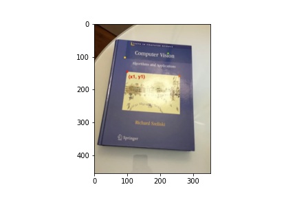
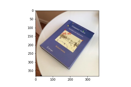
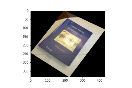
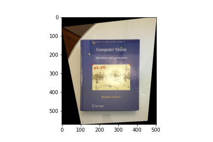
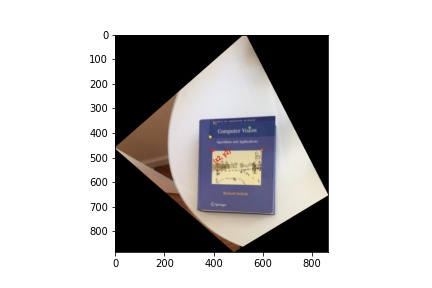
Image Rectification
Using the same images, I created rectangle coordinates and warpped the four cornors of the book to the rectangle.
Part B
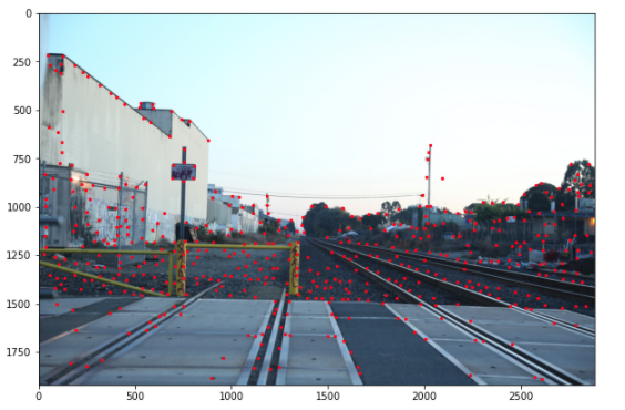
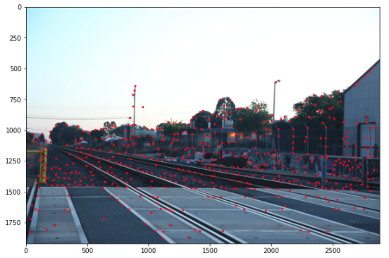
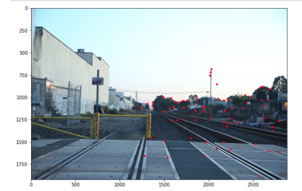
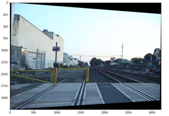
Step 1: Detecting corner features in an image
I used get_harris_corners to get the cornor points.
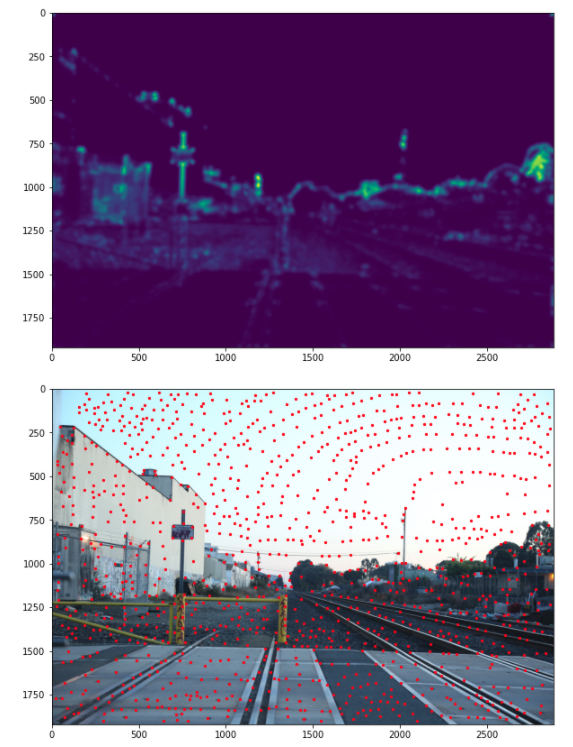
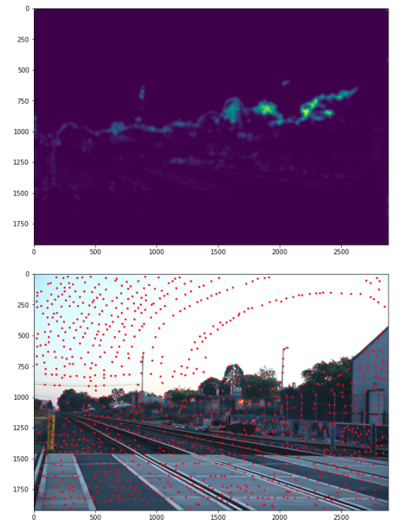
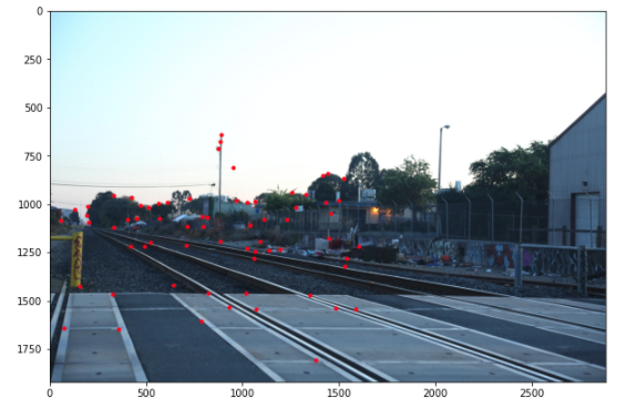
Step 2: Non-Maximal Suppression
I built the following pipeline to filter out points and make it spread out.
1. Build a hashmap, key is the coord, value is h values(value returned by corner_harris).
2. Sort the array by h values.
3. Create the matrices of vectors from the interests points.
4. Calculate the distance between the interests points by using dist2.
5. Extract the upper triangular matrix, because we only care about the distance between one interest point and the next interest point that has a higher h value.
6. Find the max distance for each interet points, which are their supression radius.
7. Build a hashmap, key is the coord, value is the supression radius.
8. Sort the interest points by their supression radius again.
9. Get the top 500.
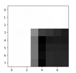
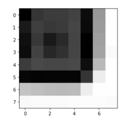
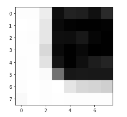
Step 3: Extracting a Feature Descriptor for each feature point
I iterated through each interest point, and used '''patch = im[pts[0]-20:pts[0]+20:5, pts[1]-20:pts[1]+20:5]''' to build the 8*8 patch with interval of 5, then normalized it.
Below are some example of the patch that shows the cornor clearly.
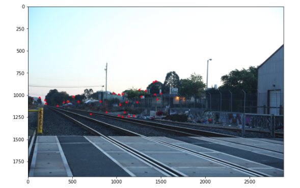
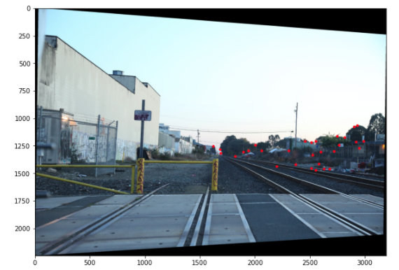
Step 4: Matching these feature descriptors between two images
I built the pipeline below to match feature descriptors.
1. I found ssd from one patch to another.
2. I then sort the ssd list and find the index of the first and second nearest neighbors
3. I calculated the ratio between the first and the second nearest neighbors.
4. I set thresholding to 0.1(according to the paper) to filter out the outliers.
Step 5: Use a robust method (RANSAC) to compute a homography
I folowed the steps introduced in lecture.
1. Select four feature pairs (at random)
2. Compute homography H (exact)
3. Compute inliers where dist(pi’, H pi ) < 1
4. Keep sample pairs, back to step 1
5. Keep largest set of inliers
6. Re-compute least-squares H estimate on all of theinliers

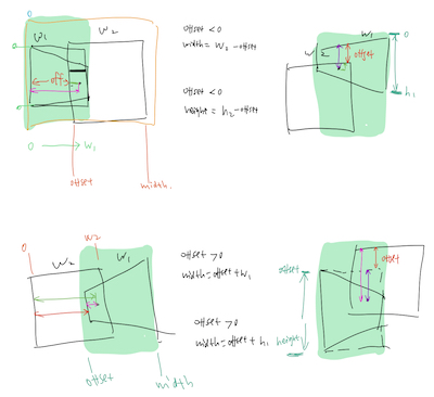
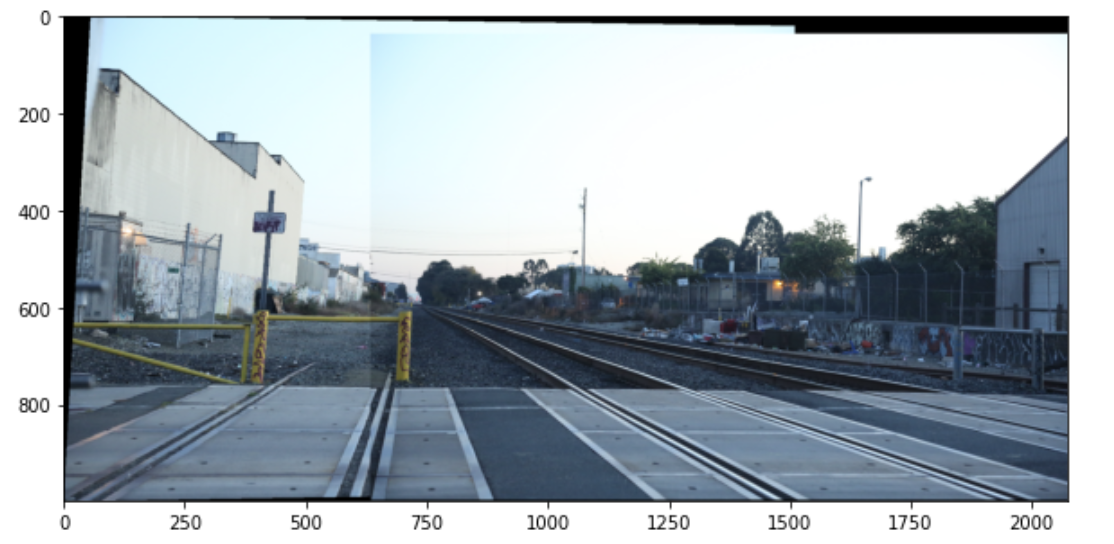
Step 6: Mosaic
This is also the last part of part A.
Fo auto stitching, to calculate the mosaic image's dimentions, I considered the 4 cases below when the weight and hight offsets are negative or positive.
For each case, I used the index range calculated below to assign the pixel values to the mosaic image.
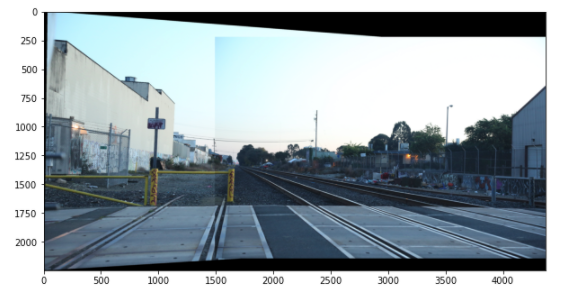
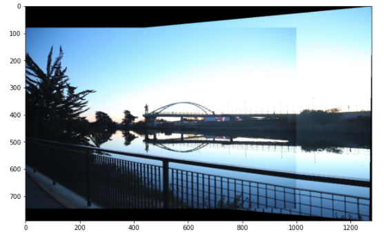
To blend the image, I used the code from project 2 to blend the above two images together. Because the images are very big, I had to adjust the size to speed up the runtime. That's the reason why the image is blurred.
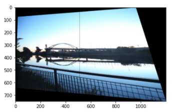
Manual Stitched
Here is the result from part A, where I picked the matching points manually.
You can see that the stitching is not accurate but the blended image still works pretty well.
Second Set of Images
Manual Stitched
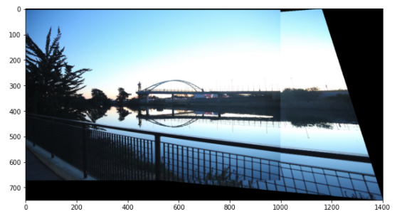
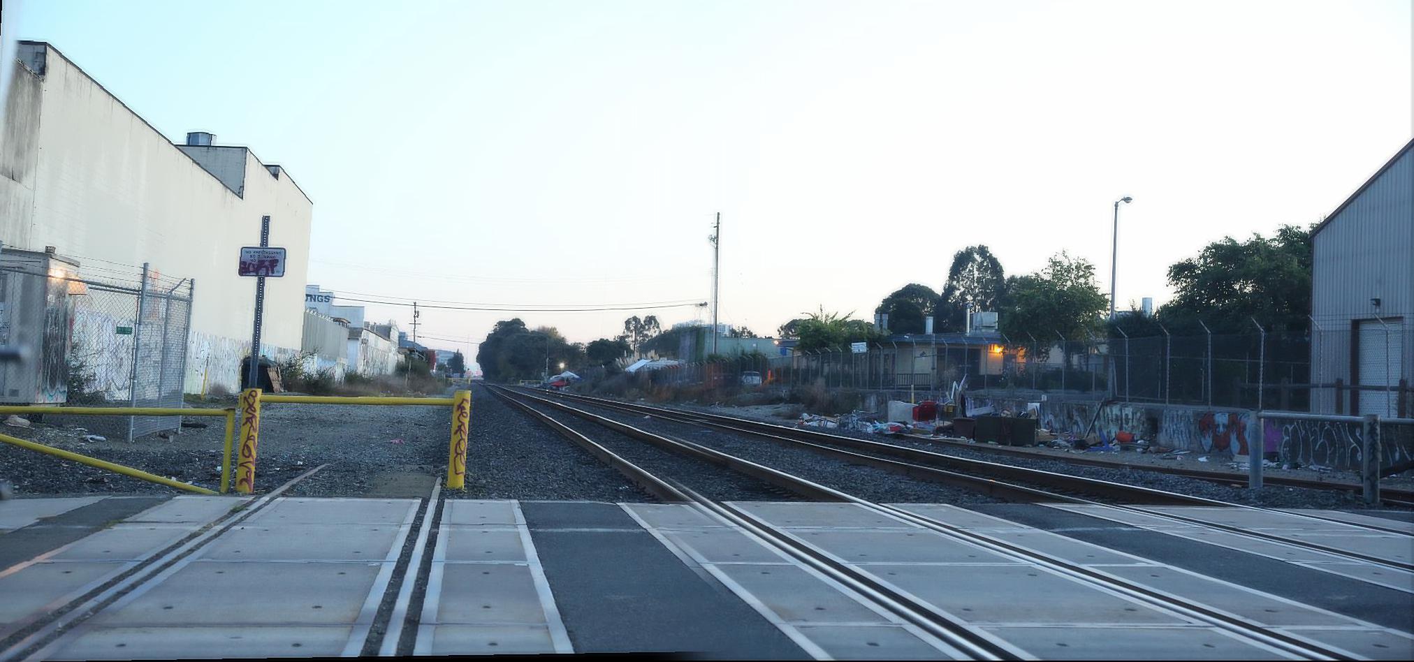
Auto Stitched
Here, the images below are much better than the manual stitched ones. Although when selecting the points I specifically chose the ones that are in the overlap region from the two images, the points I picked cannot be very precise, and that can affect the Homography I calculated.
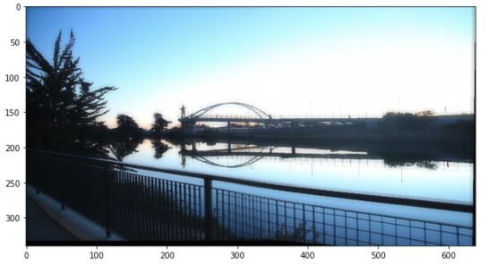
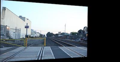
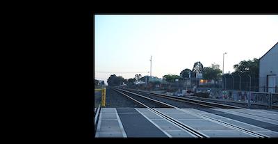
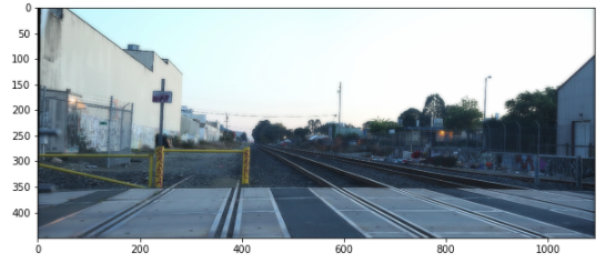
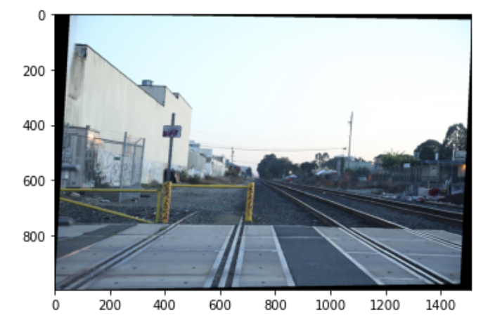
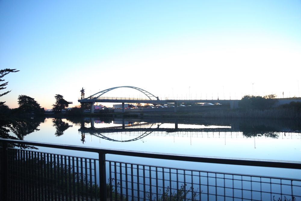
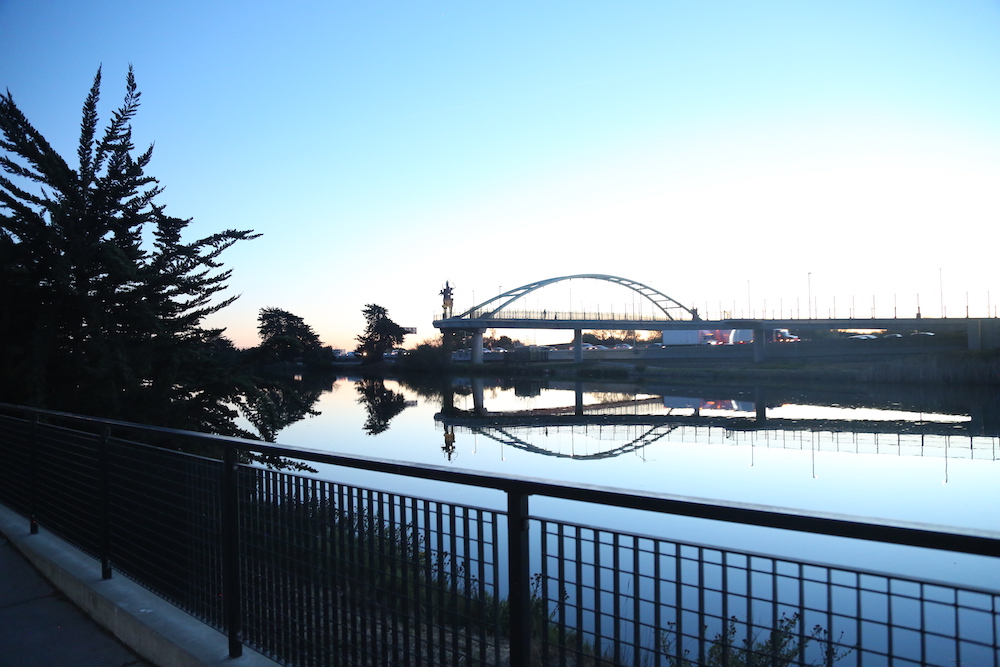
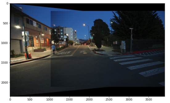
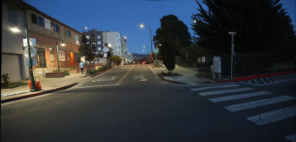
Third Set of Images
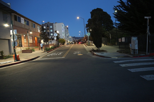
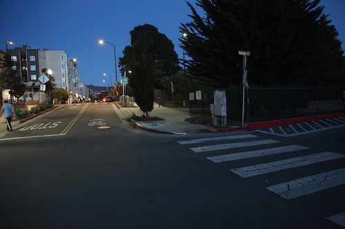
Manual Stitched
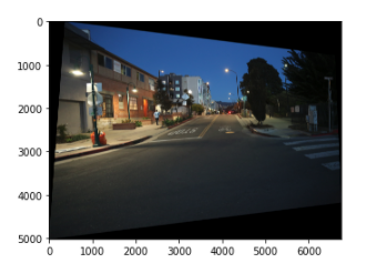
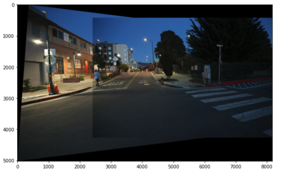
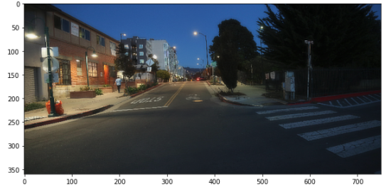
Auto Stitched
For this case, both methods worked pretty well. One fun thing is that when blending, the guy walking away from the camera is kept but not the one that passing the street.
What I've learned
This is the hardest project for me, but it's fun to see that everything worked in the end and it's amazing how well it works!