Image Warping and Mosaicing

CS 194-26 Project 5 - Fall 2020

Glenn Wysen

Example mosaic of the entrance to my apartment.

Part 1

Manual Selection and Rectifying Images

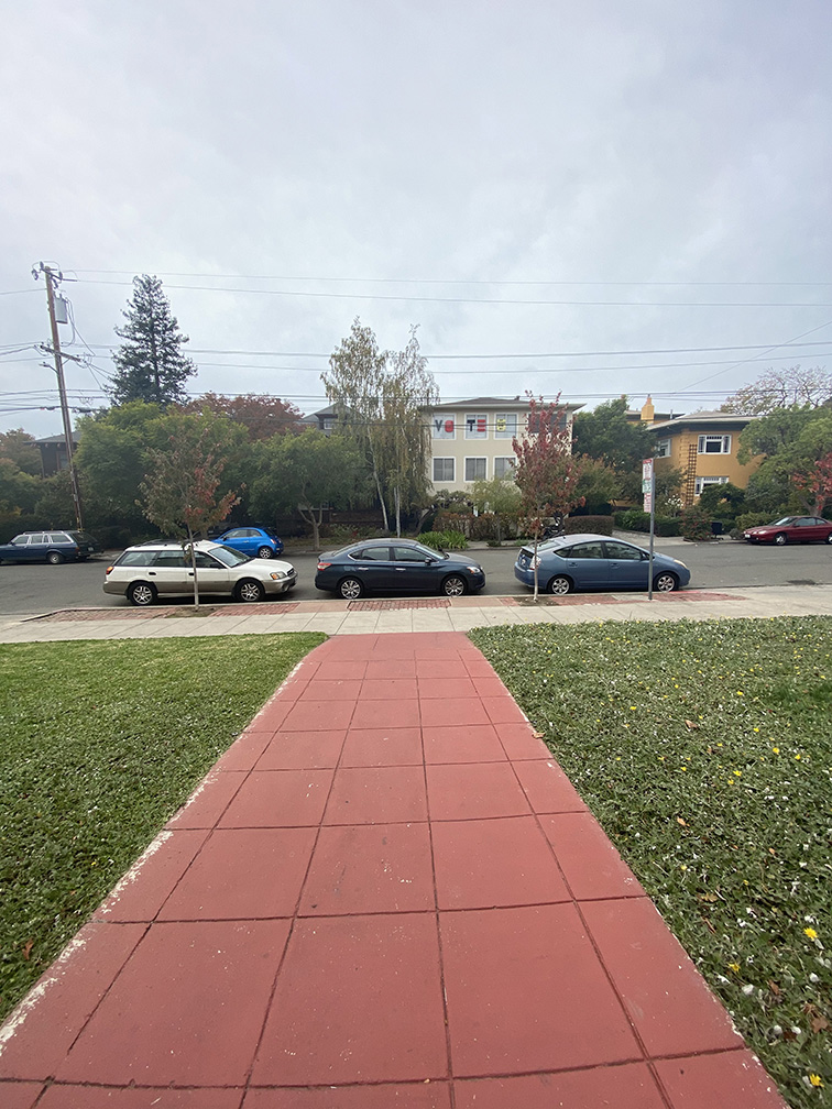
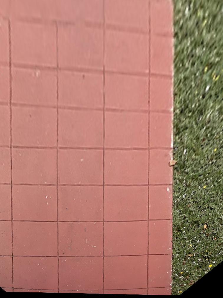
The homography matrix was calculated by taking the inputted keypoints and doing least squares to find the affine transformation that yielded the best results for all the points. Once the homography matrix calculations were done, the process of rectification became elementary. All that is needed to rectify an image is to select 4 points in the original image which are known to be in a square in real life but appear warped due to the perspective of the image. Then select 4 points in an imaginary square (ex. [0, 0], [0, 1], [1, 0], [1, 1]) and use those as the reference points for computing the H matrix. Lastly, the H matrix is applied to the points in the original image which results in the rectified image shown below.

Fig. 1 - Two images after the left has been warped and blended with the right using manual keypoint selection.

Fig. 2 - Image before rectification.

Fig. 3 - Image after rectification.

Part 2

Detecting corner features in an image

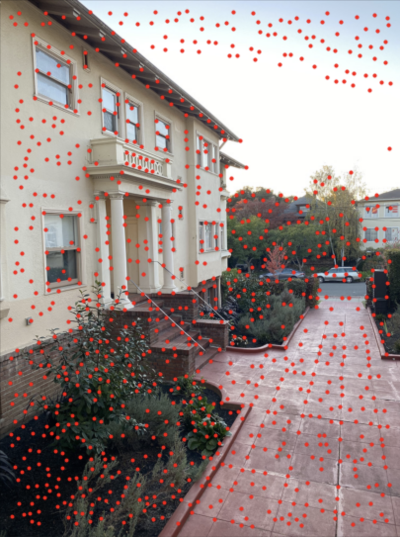
This step was provided as a template function for finding the Harris corners of an image on the class website. An example of Harris corners plotted over an image is shown in Fig. 4. The only tricky part about this was editing the min_distance attribute so that there were not too many points. I changed that value from 1 to 10.

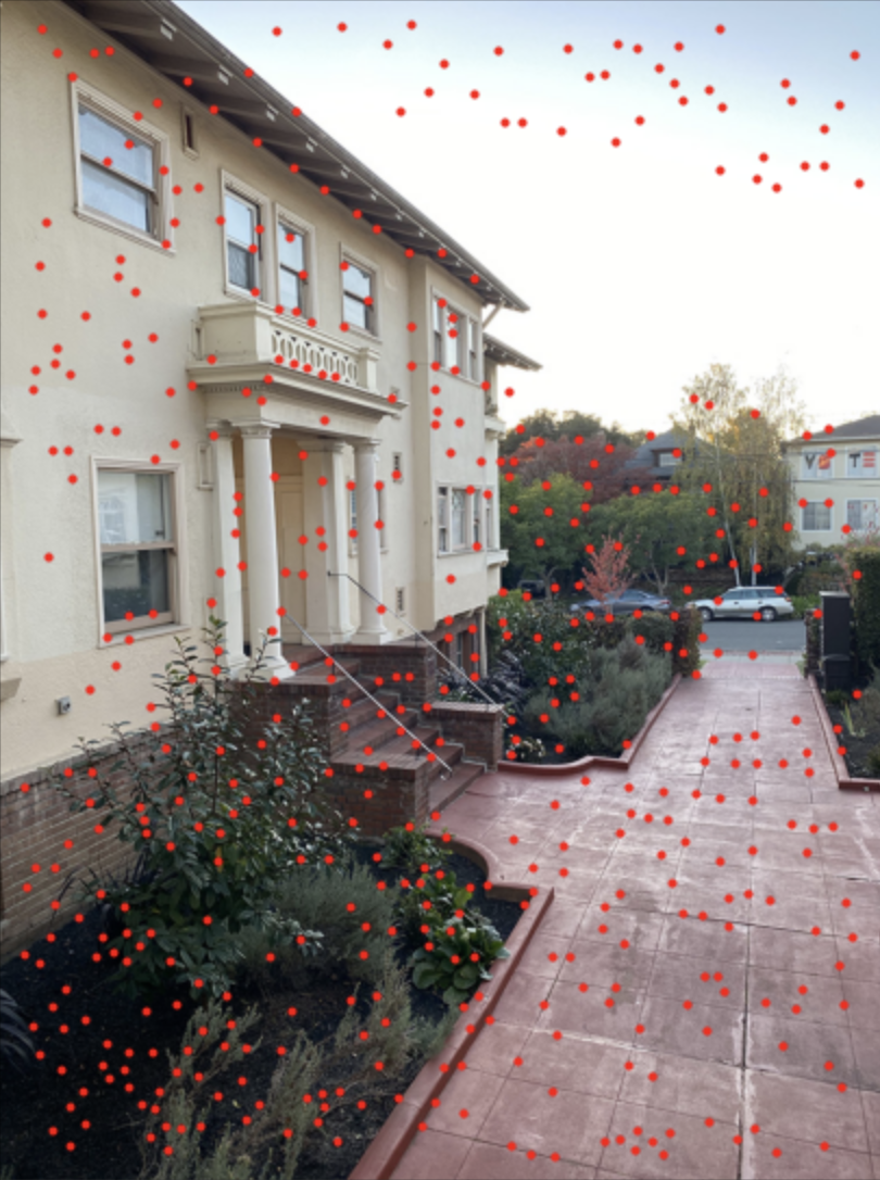
Fig. 4 - Example image with Harris points plotted over.

Fig. 5 - Harris points after undergoing suppression.

Adaptive Non-Maximal Suppression

At this point there are too many close together Harris points and we only need to keep the best ones and have them be more spread out. To do this I implemented an Adaptive Non-Maximal Suppression algorithm to determine how "corner-y" the corners are and only keep the best 500 points. The suppressed points are shown in Fig. 5

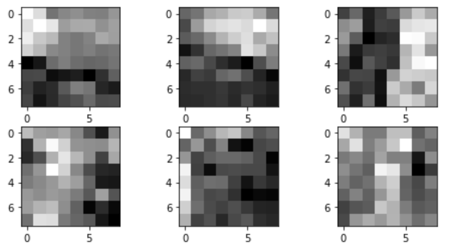
Extracting Feature Descriptors

Now that there are less points, the next step was to find a feature image for each point in order to match them later. For this step, I took a 40x40 window around the point, applied a gaussian blur to the patch, and then downsampled to an 8x8 patch. Each of these patches was stored with its corresponding point for matching later.

Fig. 6 - Some examples of 8x8 feature patches.

Fig. 7 - Harris (red) and matching (blue) points from the left image.

Fig. 8 - Harris (red) and matching (blue) points from the middle image.

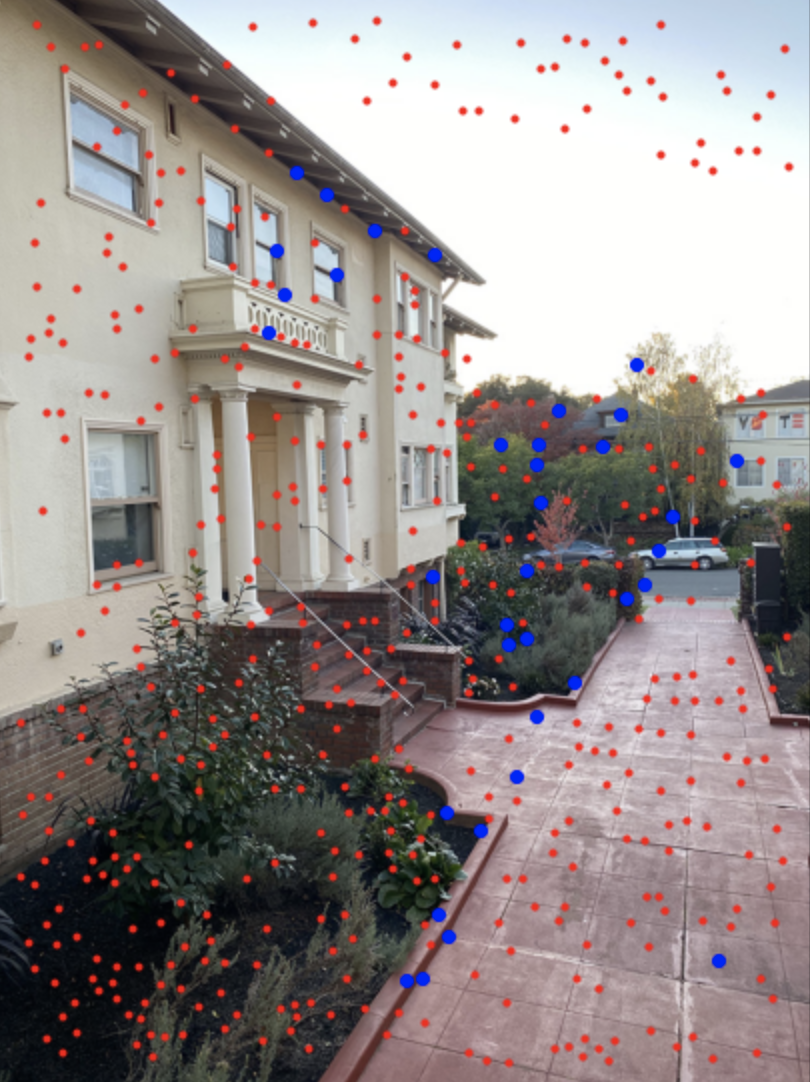
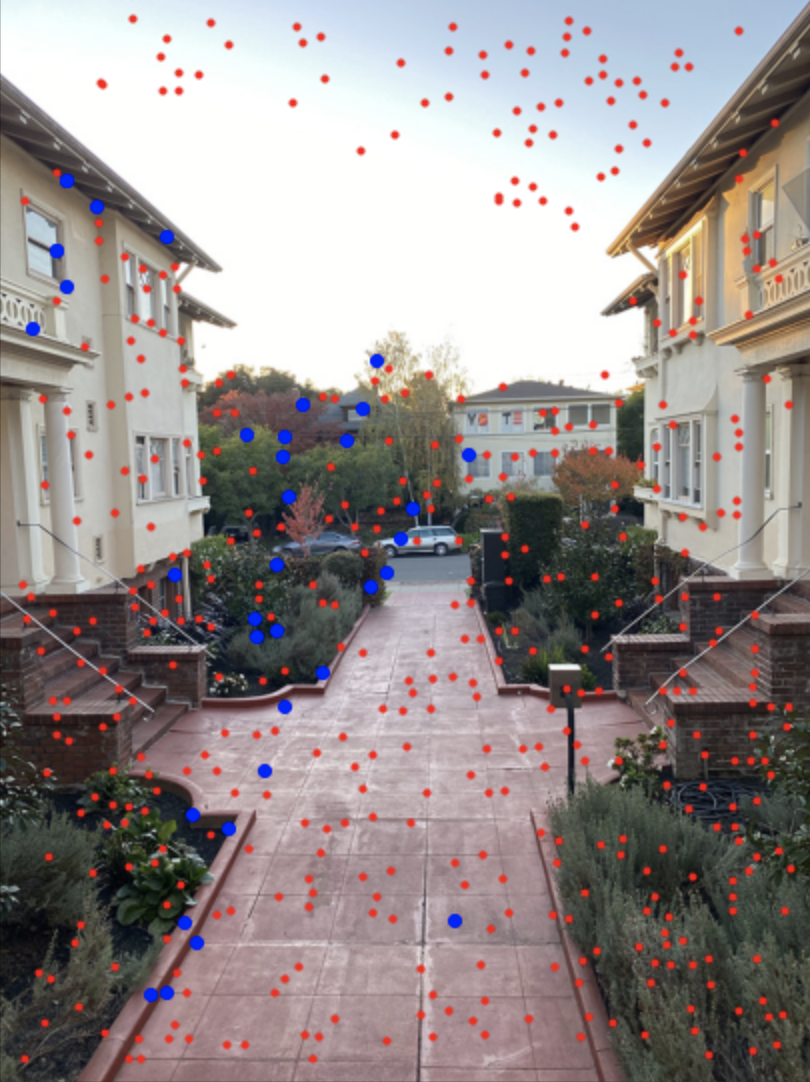
Feature Matching

Feature matching was accomplished by taking the set of features from each of the two images to be stitched and for each feature in the first image, finding the closest and second closest features (using SSD) in the second image. To weed out outliers, only the features that had a ratio of closest:second closest less than 0.2 were used (i.e. only the features who only had one close match in the second image). Two images with their suppressed Harris points in red and matching points in blue are shown in Fig. 7 and Fig. 8.

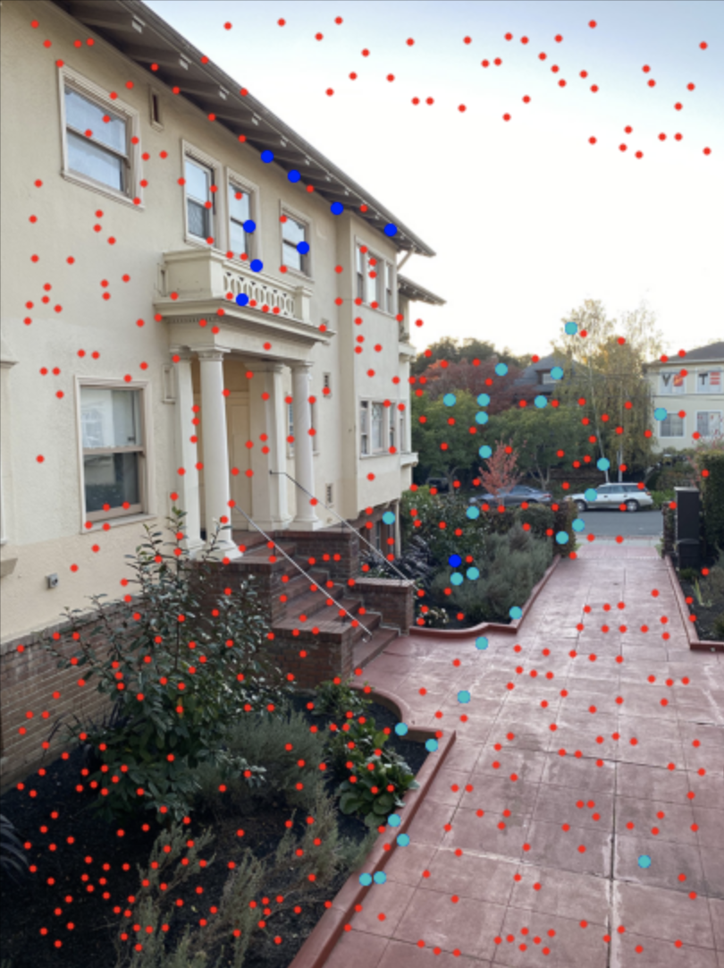
Using RANSAC to compute a homography

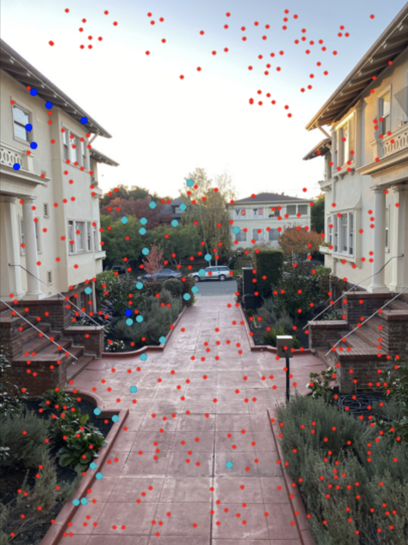
We are close to having enough points to compute a homography, but there are still some that are not perfect. Enter RANSAC. I repeatedly randomly selected 4 matching points to compute a homography then warping all the points and calculating how many inliers (points that fall within 2 pixels of where they are supposed to) there were. I found that after 1000 random selections my algorithm would usually find the four points that worked the best. After these points were found, a homography could be calculated using least squares on all the points that were inliers from the transformation. Fig. 9 and Fig. 10 show the original suppressed Harris points in red, the matching points from feature matching in blue, and the final RANSAC matching points in cyan.

Fig. 9 - Harris (red), matching (blue), and matching after RANSAC (cyan) points from the left image.

Fig. 10 - Harris (red), matching (blue), and matching after RANSAC (cyan) points from the middle image.

Final Results

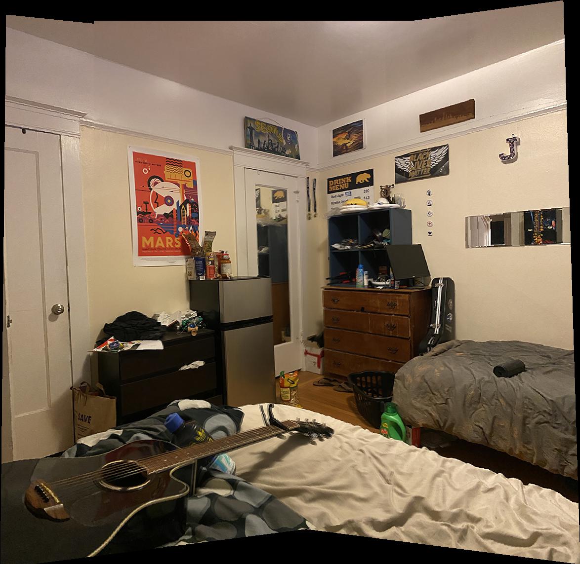
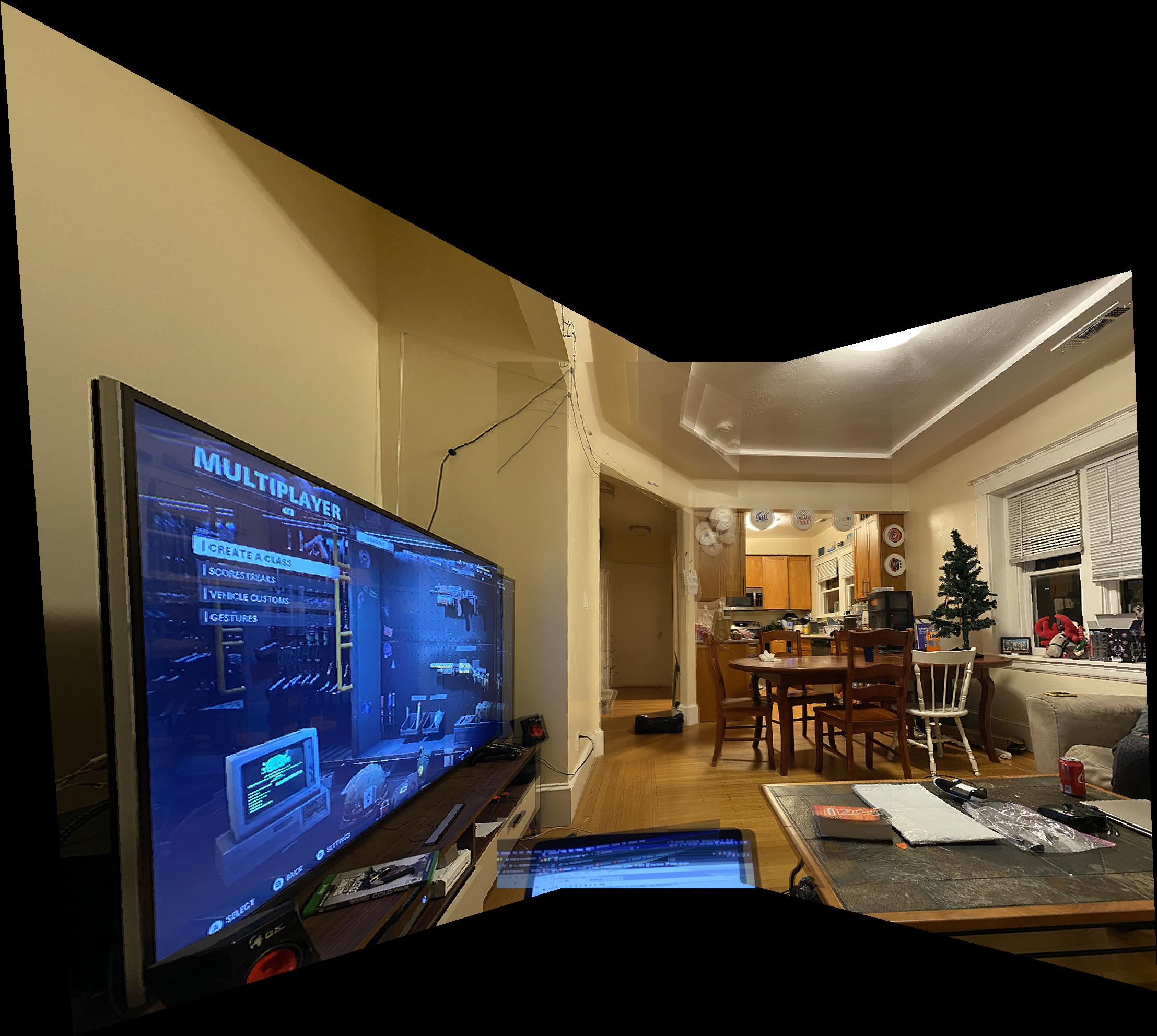
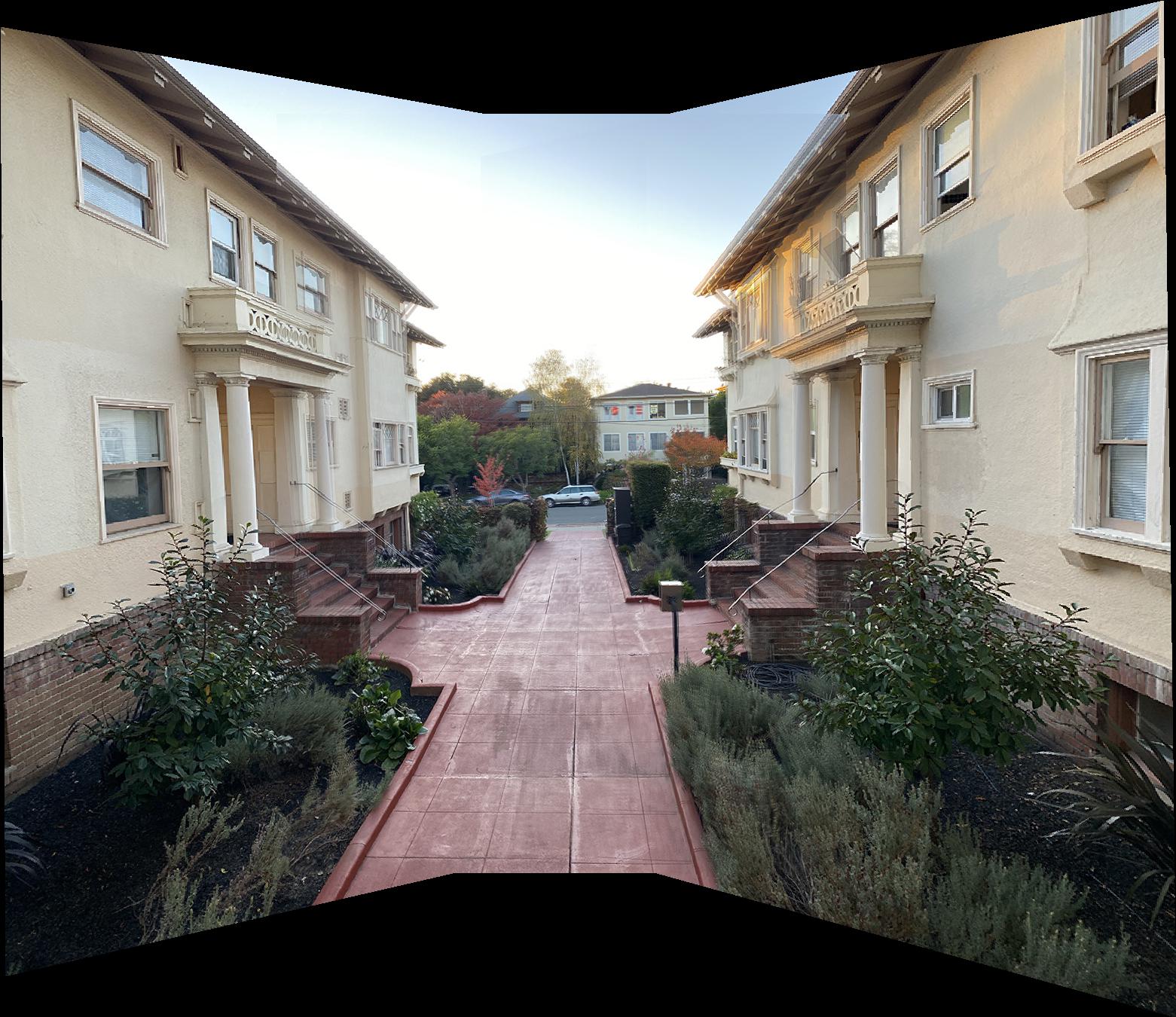
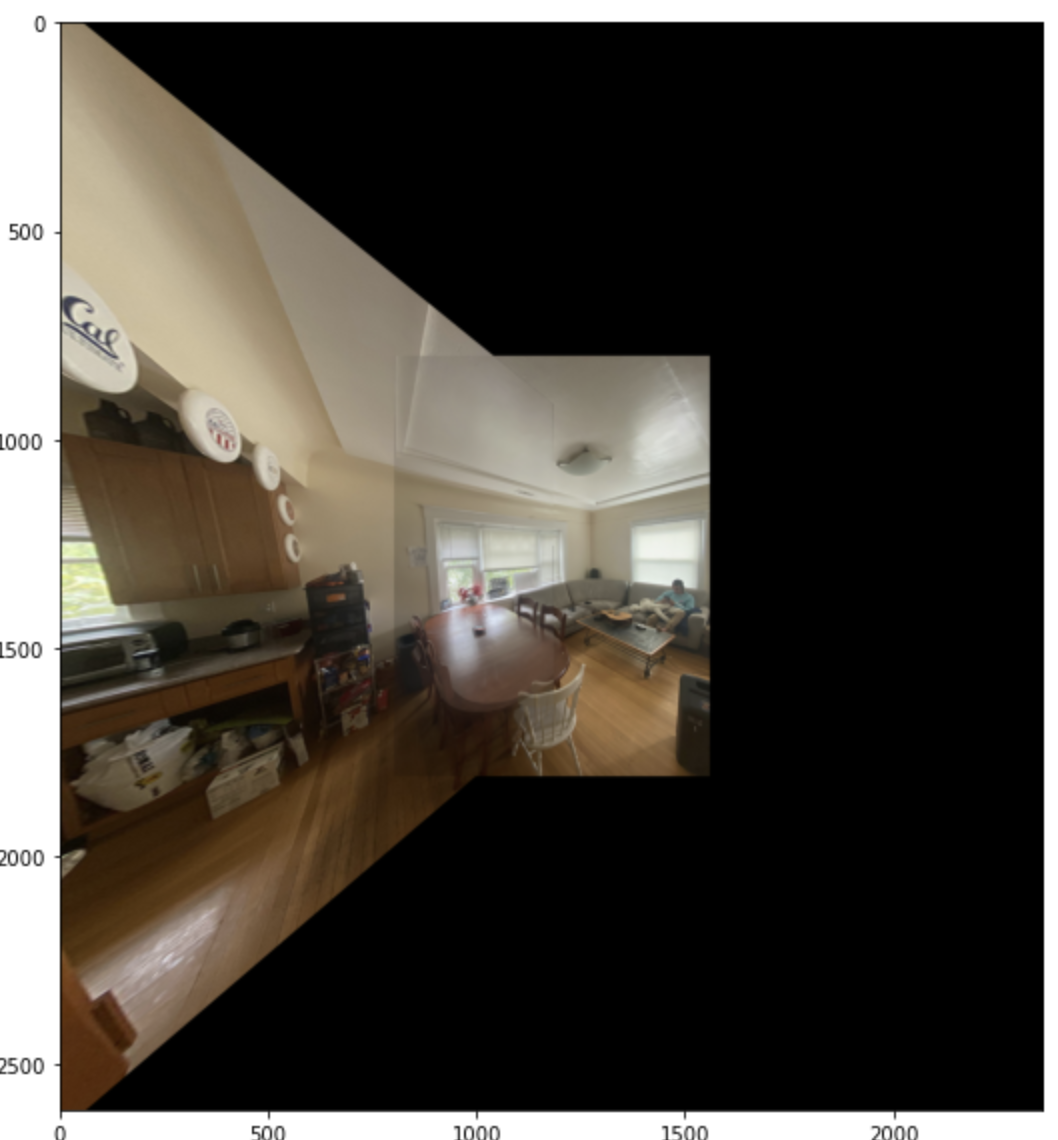
The images I took for the first hand selected point mosaic ended up being too far apart such that their features weren't matching because they looked too different. To adapt to this, the images I used for auto stitching are less rotated from each other than the first set of images.

Fig. 11 - Example mosaic of outside my apartment.

Fig. 11 - Example mosaic of my bedroom. Note that the alignment is very good as the original images were not rotated that much from each other.

Fig. 11 - Example mosaic of my living room. Note that the matching works less and less well the further away from each other the images are.