This project involves calculating a homography matrix in order to warp images into a different shape.
Shoot the Pictures
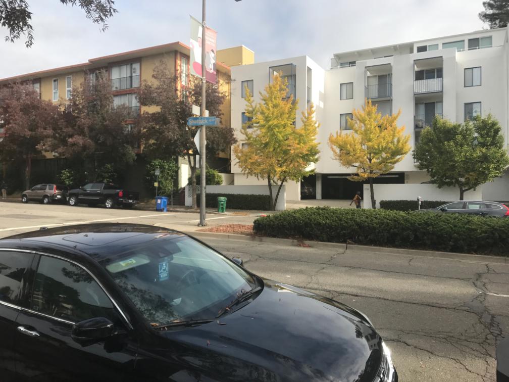
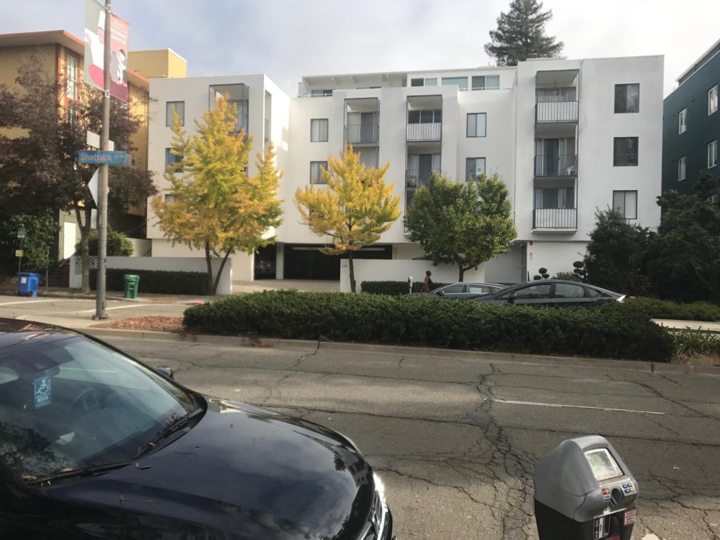
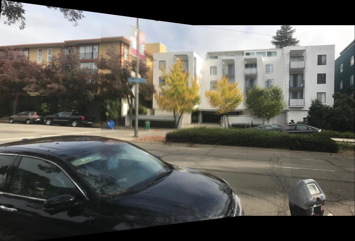
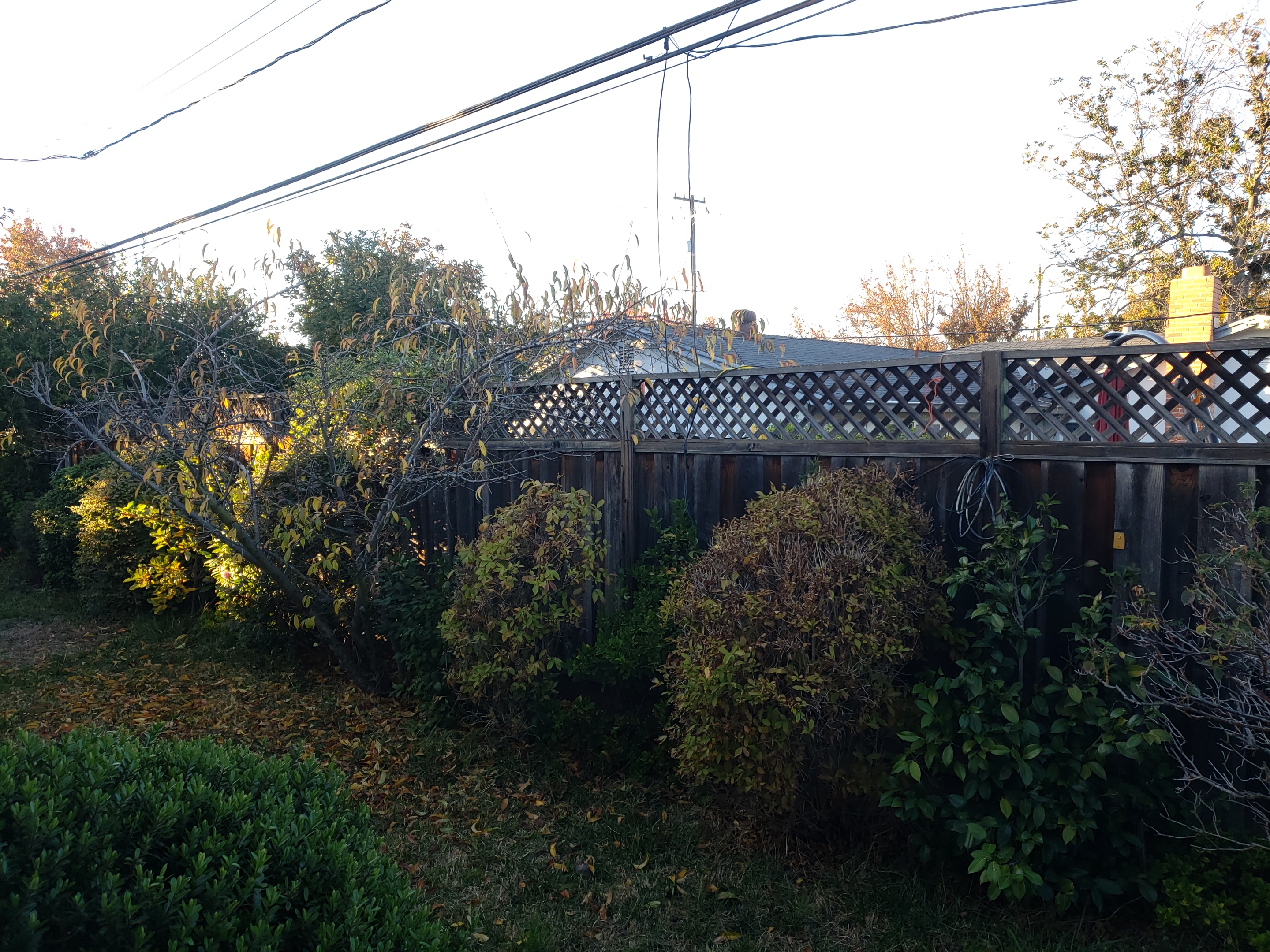
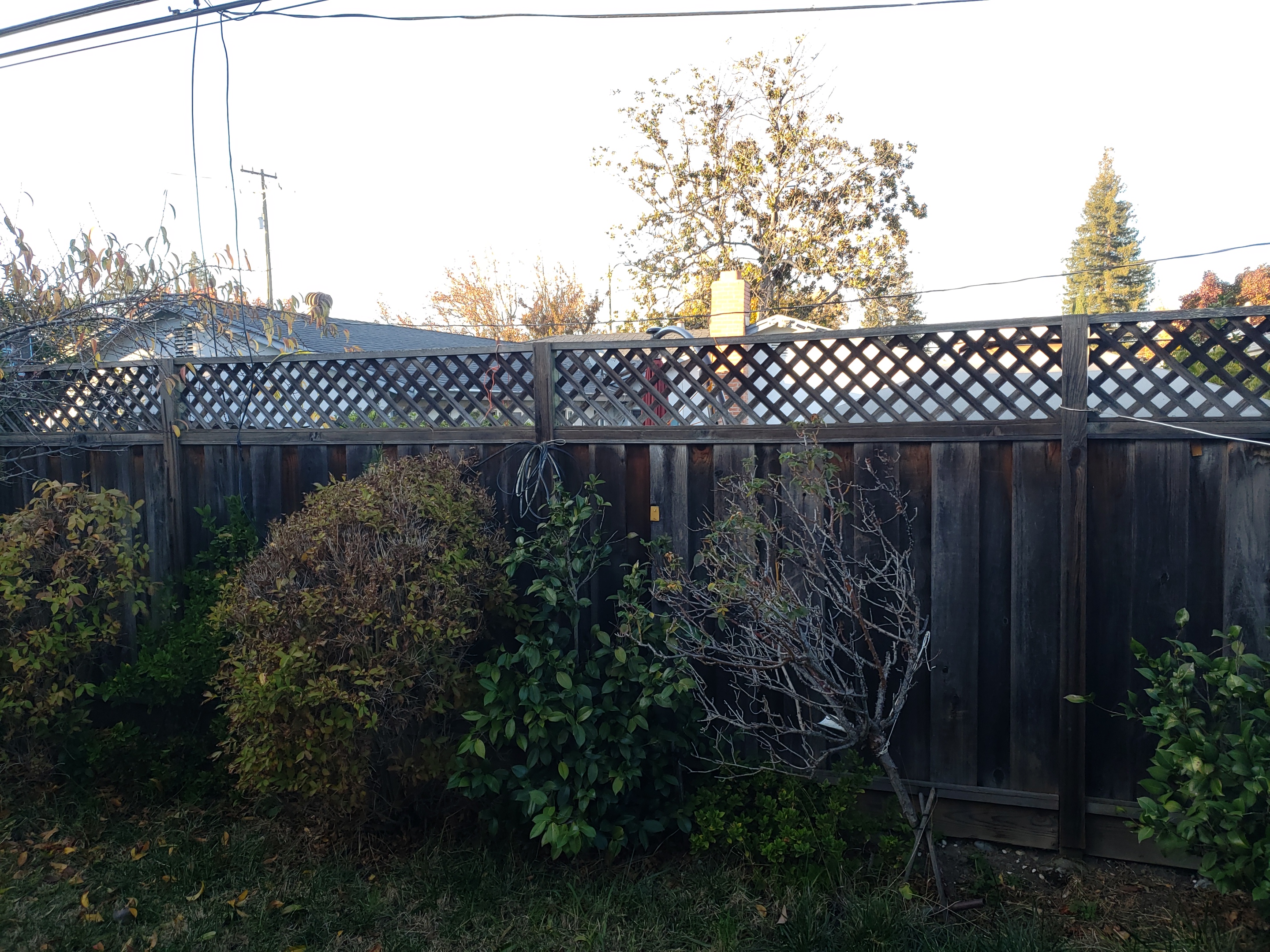
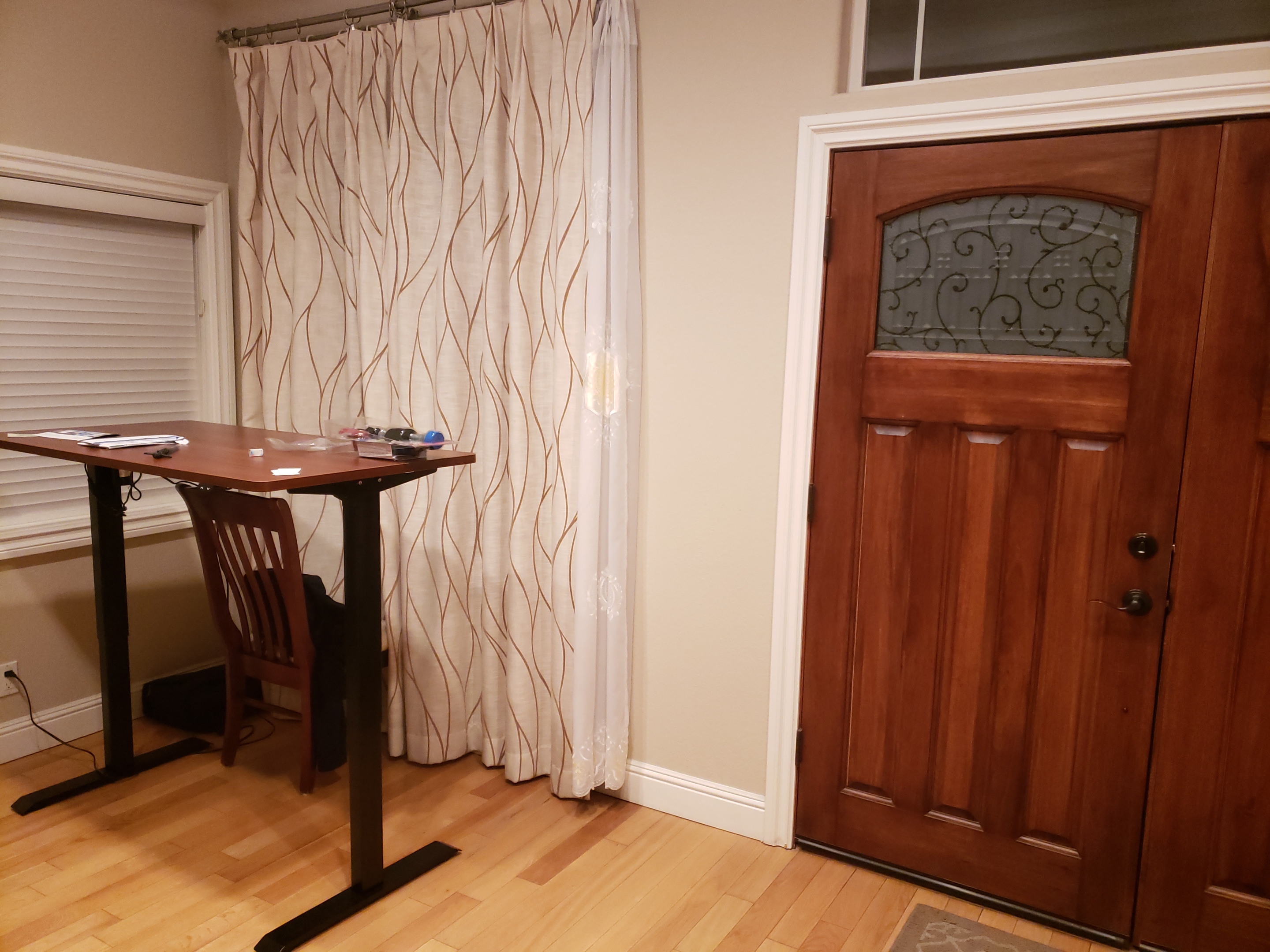
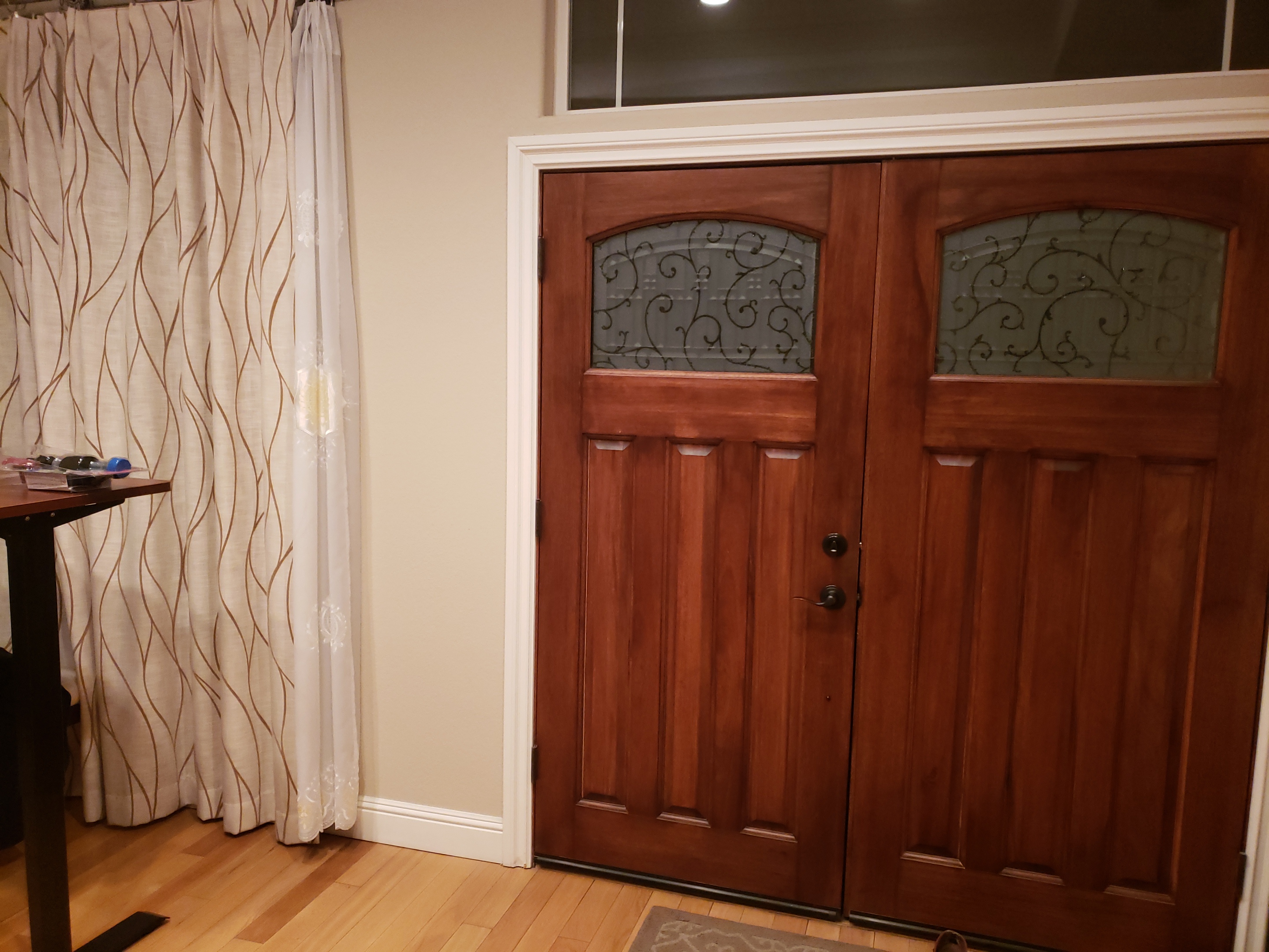
For this part I started with some sample pictures I found of Shattuck at Berkeley. They are taken from the same position with each image taken from a different rotation on that position.
Left most imageRight image
Recover Homographies
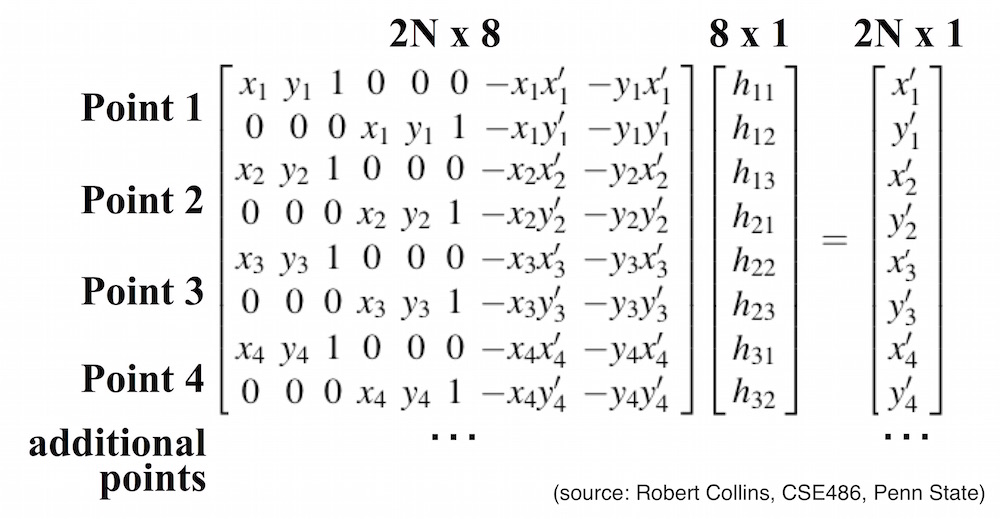
There are 8 degrees of freedom for a homography, so the homography matrix is represented by a 3x3 matrix, with a constant of 1 at the very end. The matrix is supposed to be a solution to the equation p' = Hp. To calculate the entries of the homography matrix, H, a system of linear equatinos is set up as shown below.
A system of linear equations that will be solved with least squares
Warp the Images
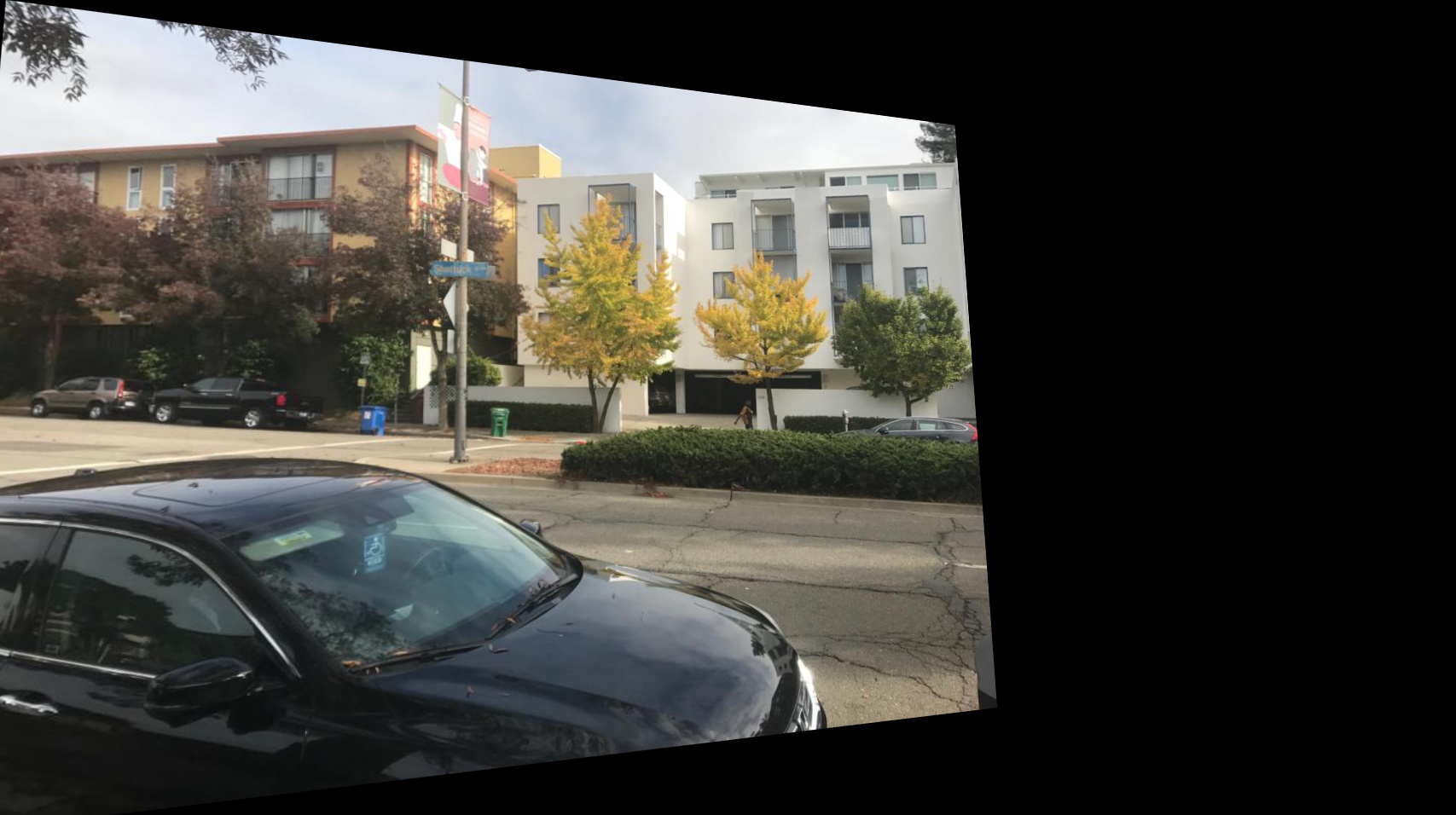
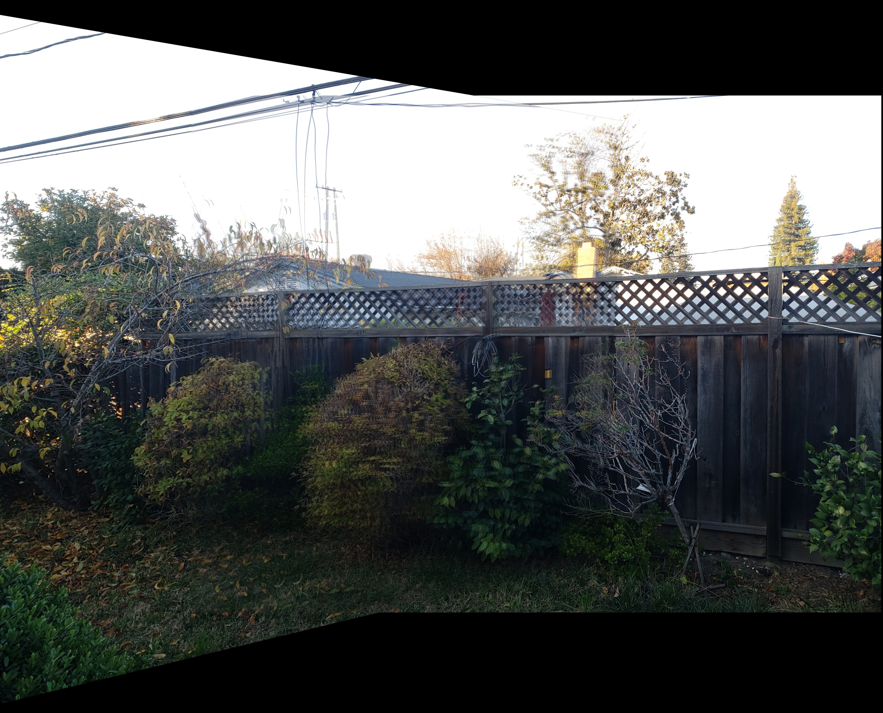
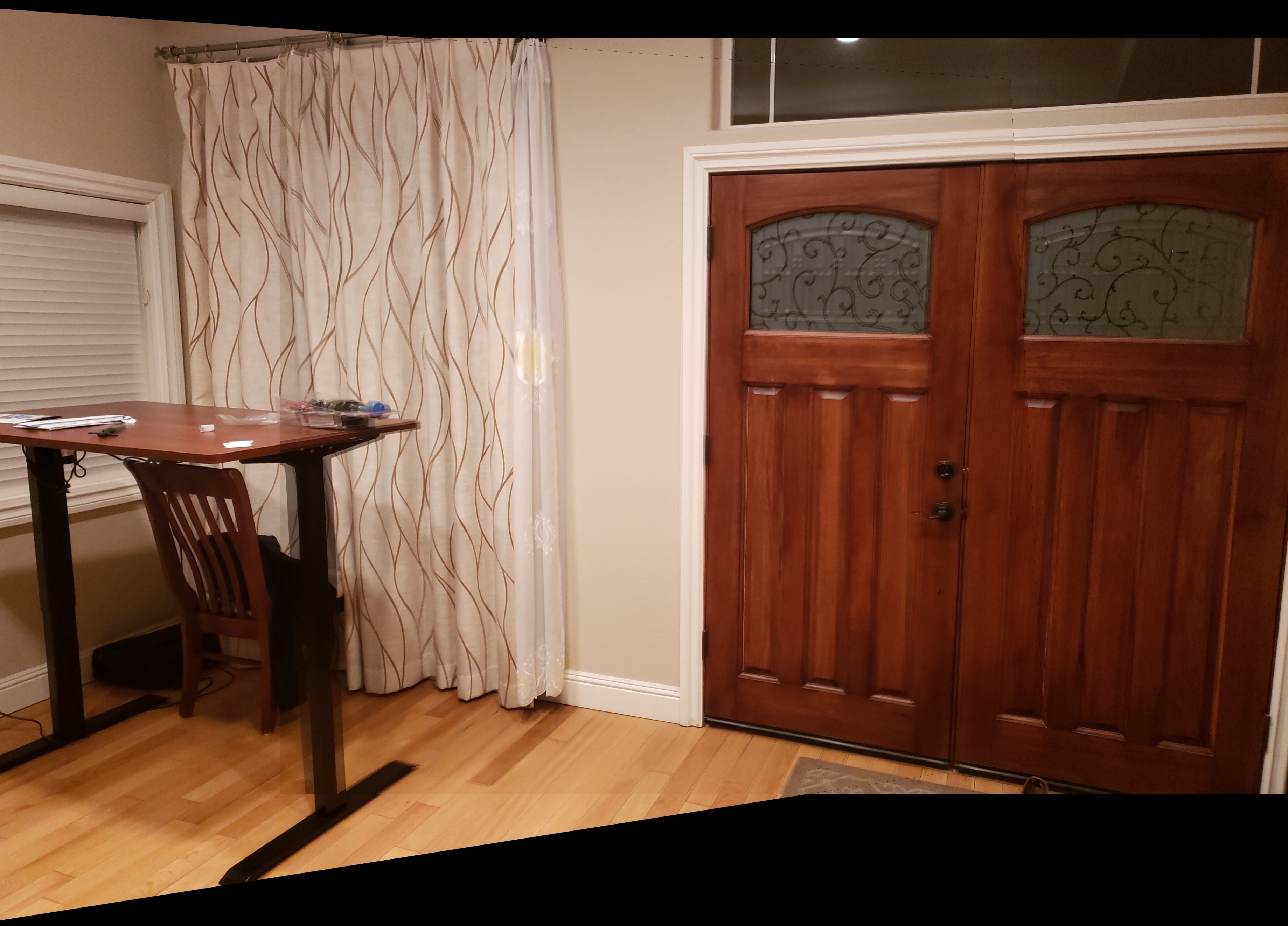
The resulting H matrix can be used with remap in order to warp images with interpolation. The warped image may be larger than the original, so padding was added to the image to account for this. 6 points from both images were selected to calculate the homography. The left image was warped to the points from the right image, so the right image stayed the same.
Left image warped
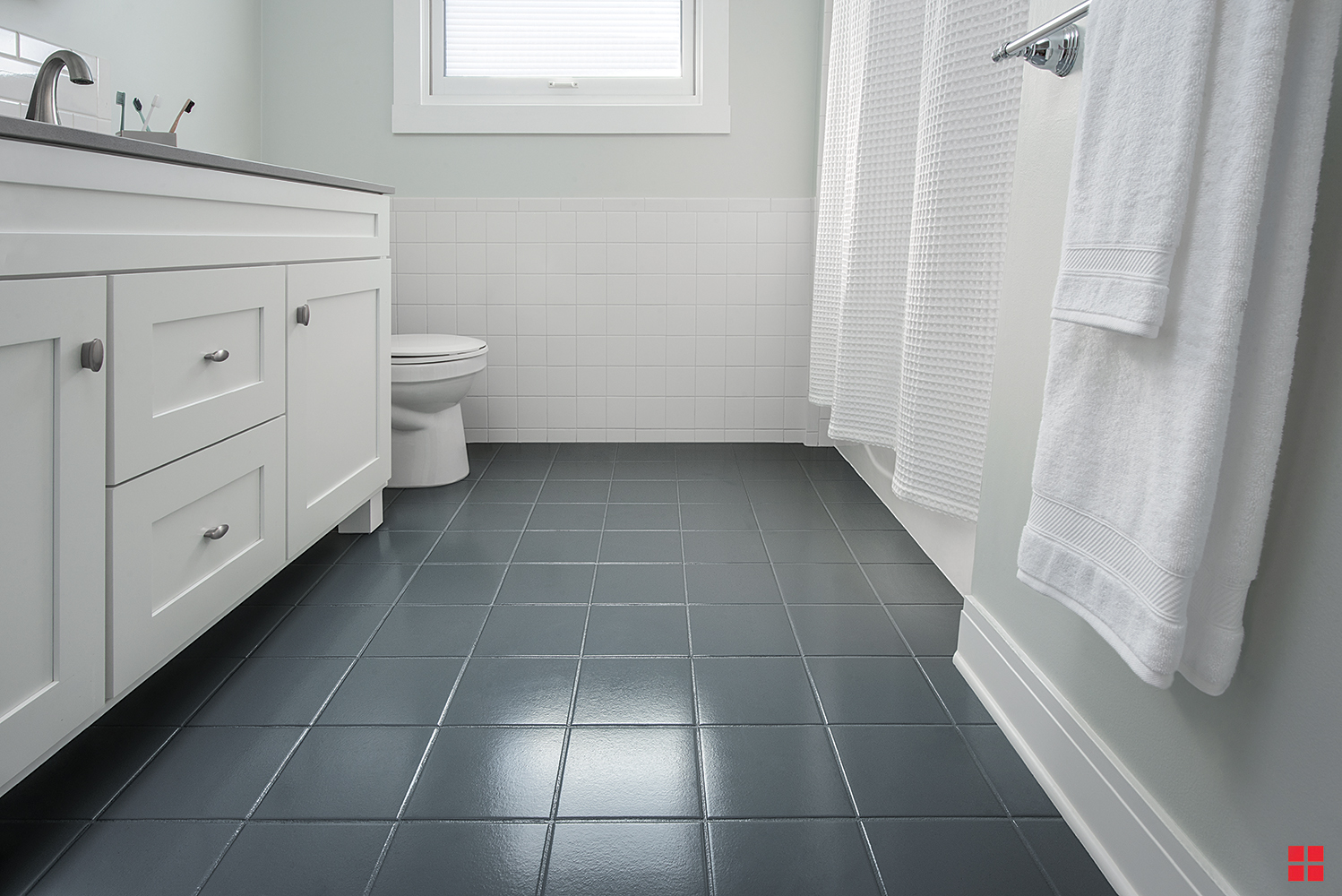
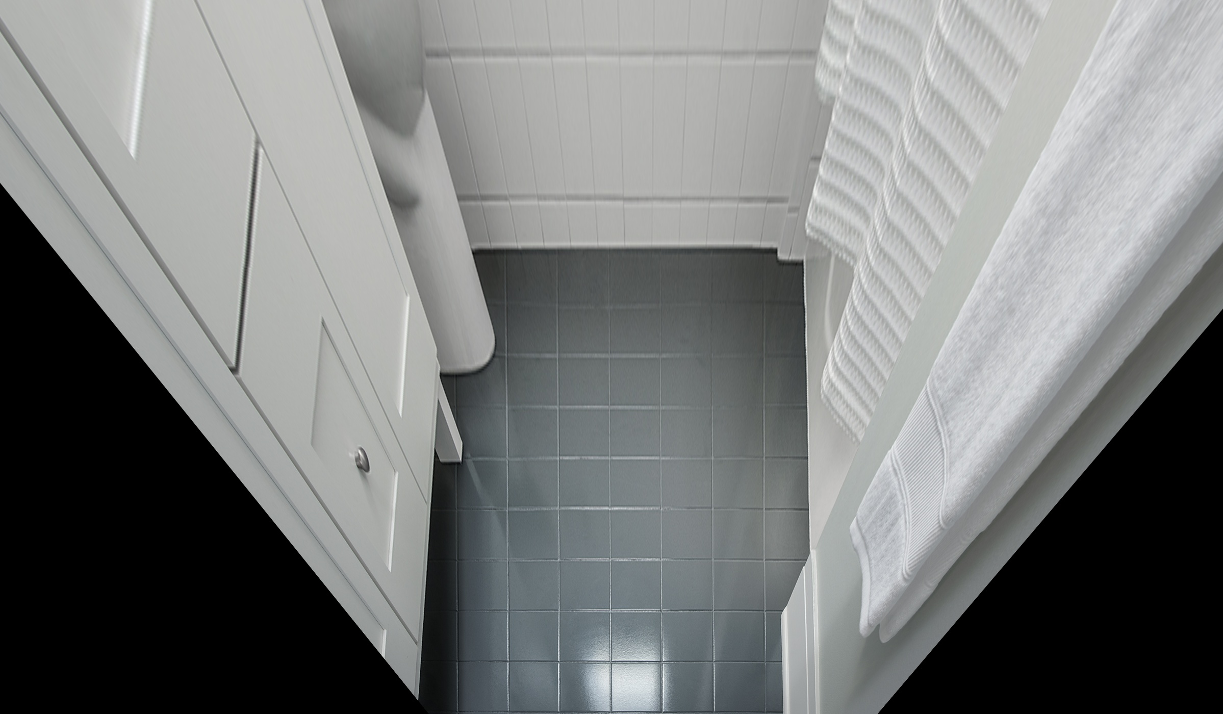
Image Rectification
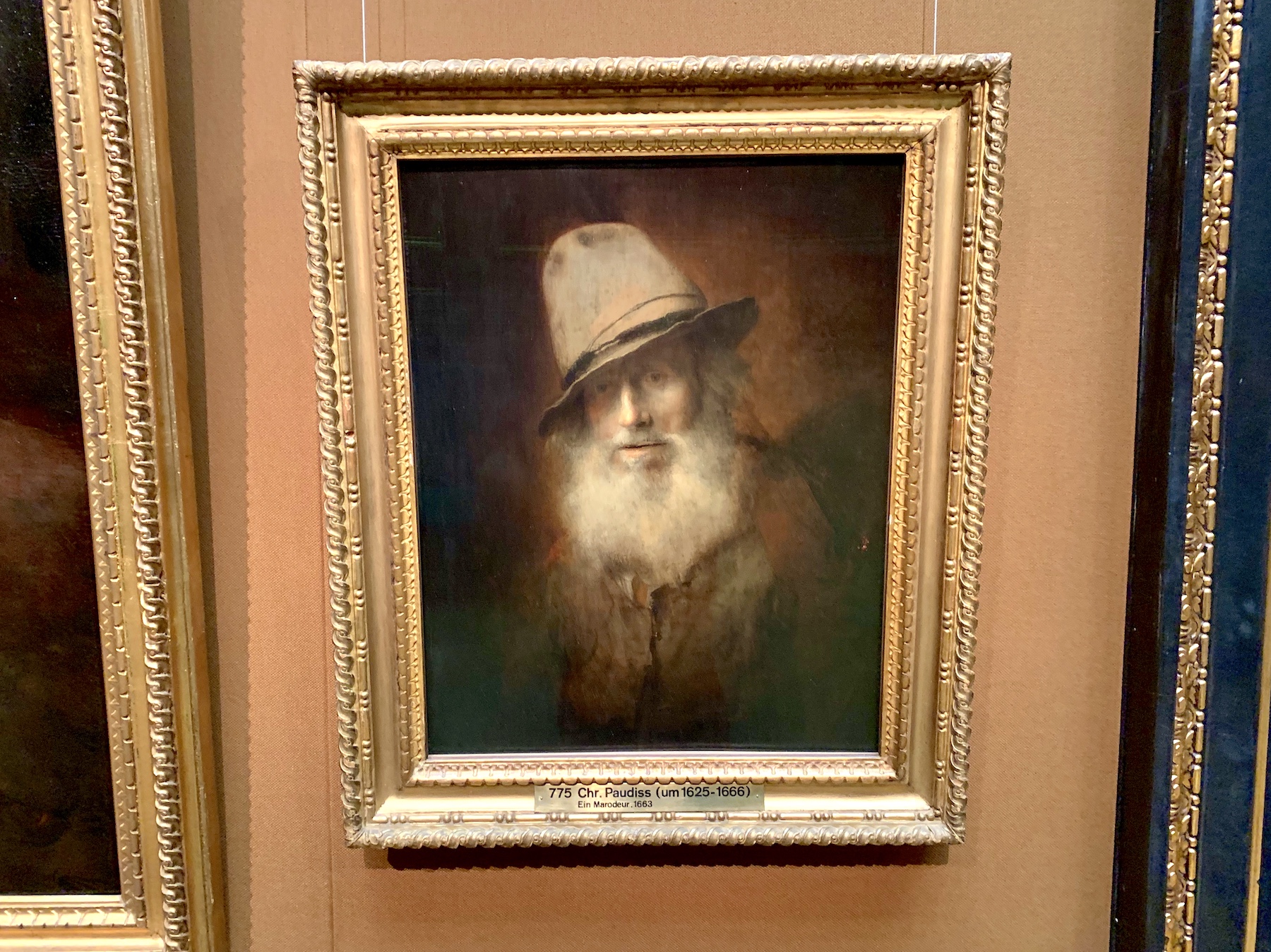
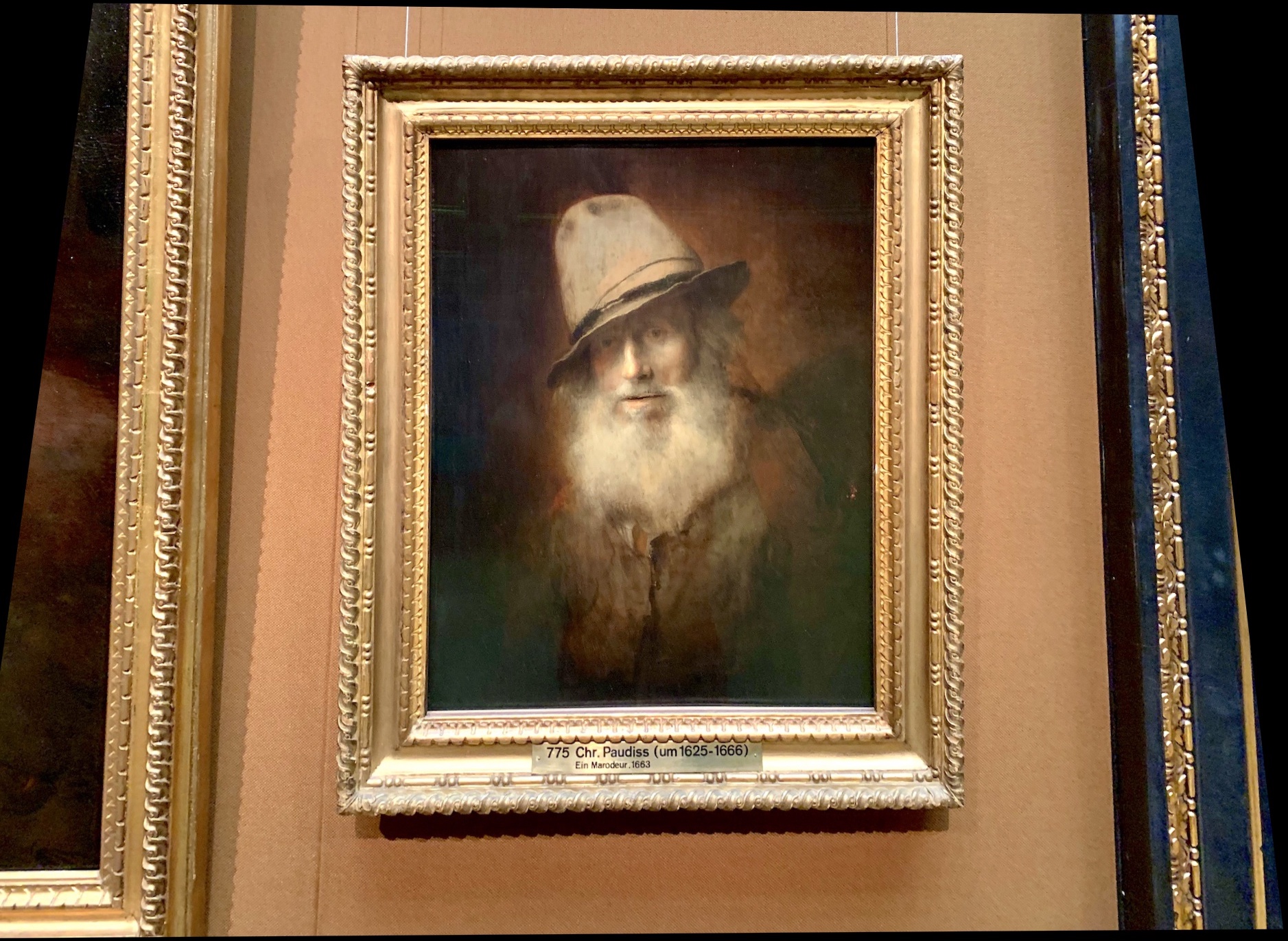
To test if my warping function was working properly, I took a few image with planar objects and "rectified" them by defining an arbitrary corresponding set of points to create a homography for. For the tiles example, I knew the tiles were square in shape, so I selected four points encpasulating a square section of the ground and calculated a homography to an arbitrary square. The painting example used the same logic, selecting the four corners of the painting and calculating a homography to an arbitrary rectangular shape of around the same proportions.
Original imageRectified tiles image based on the groundOriginal imageRectified painting image
Blend the Images Into a Mosaic
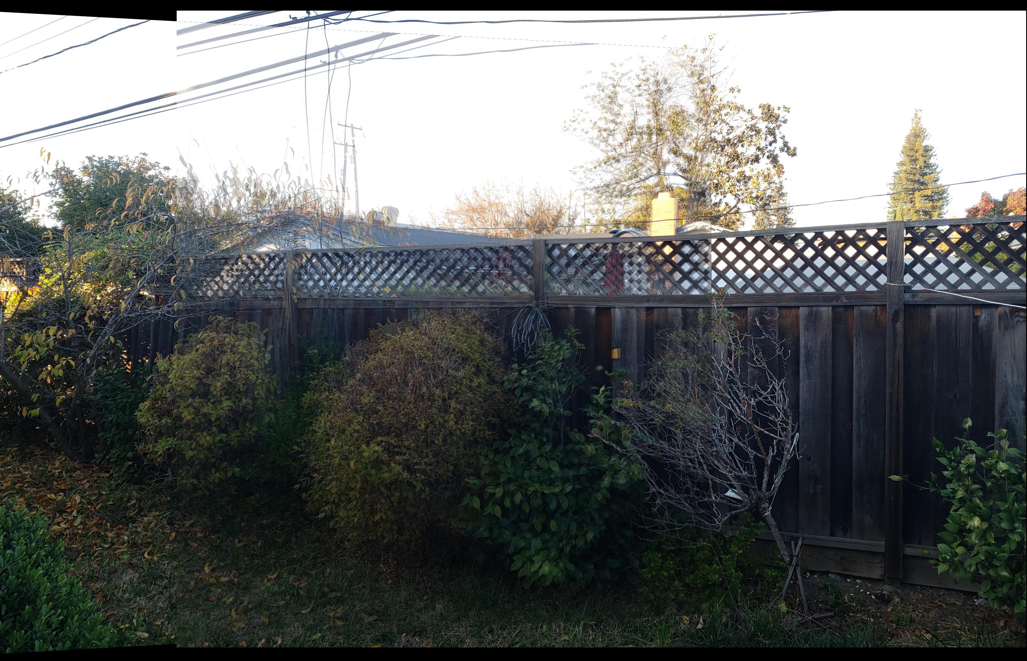
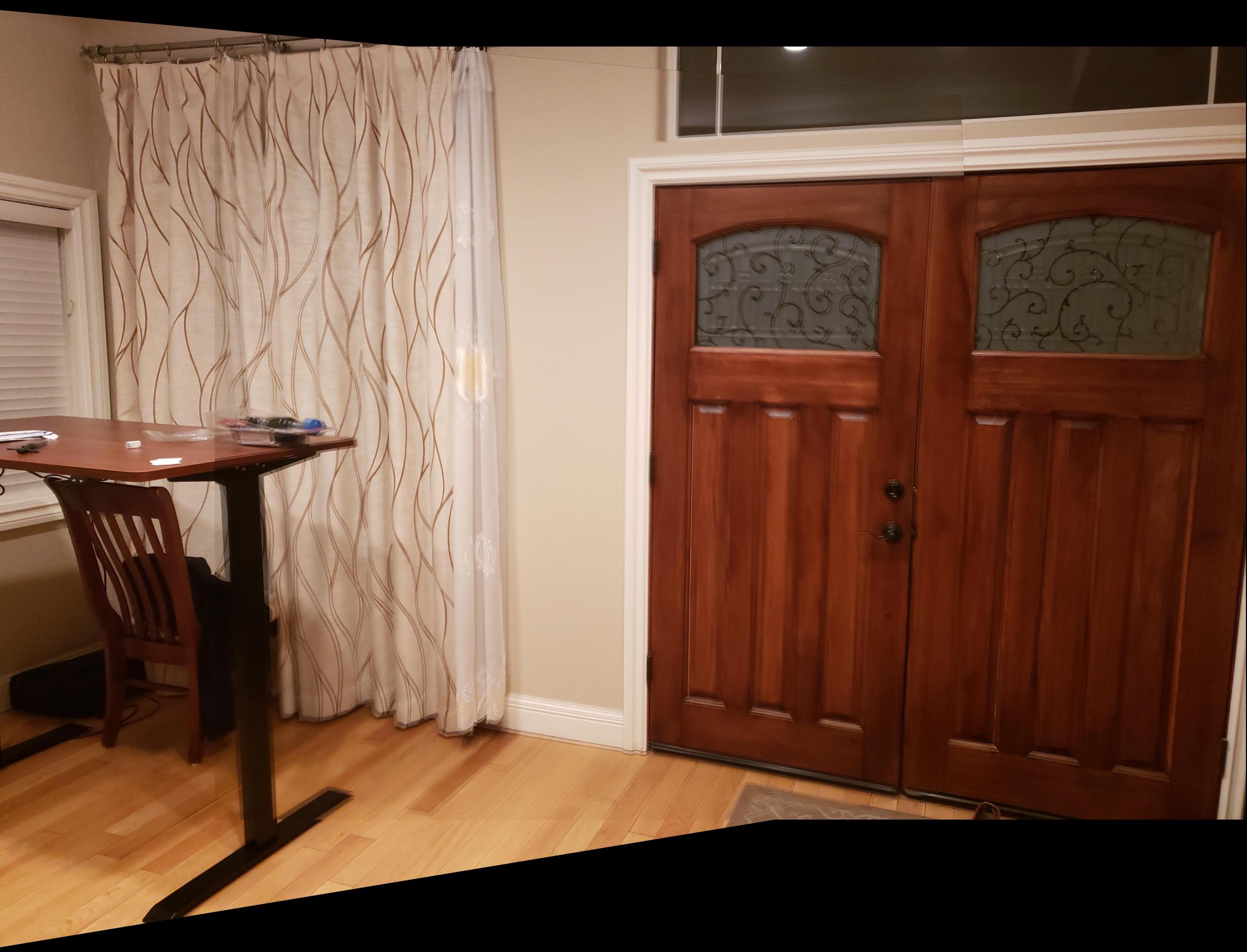
This next part was a bit trickier. Since the resulting image from the homography could fit outside the original image dimensions, padding was added to the two original images. This way if the result was shifted it would still be within frame. To calculate the homography, the indices of the new image were mutliplied with the inverse of the homography obtained earlier in order to obtain the corresponding coordinates of the source image to pass into cv2.remap that would do the interpolation.
Below is the left warped image blended with the right image, which is unchanged.
What I've Learned
This project really helped me understand the uses of homography as well as how to compute the homography matrix. Warping was a bit more difficult, but it was a rewarding seeing how the homography matrix played into retrieving the source coordinates.
Project 5B: Feature Matching for Autostitching
Overview
This is a follow up to Part A. Instead of manually choosing the corresponding points in both images, we want to be able to automatically detect corner points while also identifying matching pairs between images.
Harris Point Detector
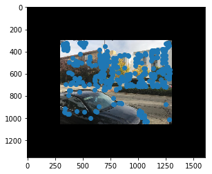
The Harris Point Detector detects corners within an image. Below is a plot of all the points plotted on a sample image. Padding was added for similar reasons as the images in Part A.
Adaptive Non-Maximal Suppression
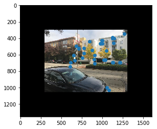
The Harris Point Detector often outputs hundreds if not thousands of corner points. This is too much to do feature detection, so adaptive non-maximal suppression is used to reduce the number of points. It looks at the radius of each points, computed as the minimum distance to a point that is significantly stronger based on a function. The points are then sorted based on their radius size, and the largest points taken to guarantee that points are not clumped together while also preserving strength. Below is the same picture after applying Adaptive Non-Maximal Suppression and getting the top 400 points.
The difference is not very noticeable as the image produced isn't very large and there were not that many points to begin with.
Feature Matching
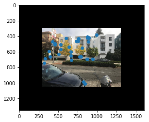
The next step is to know which points/features correspond to each other in the two images. This is done by sampling an 8x8 square around the points and finding the best matching ones as pairs. No rotation variance was applied, and the descriptors were biase/gain-normalized. Here are the two sample pictures from Part A with the remaining poitns after feature matching.
RANSAC
After finding the corresponding features, the final step is to perform the RANSAC algorithm. The algorithm consists of taking random sets of 4 points, calculating a homography, and calculating the number of inliers per iteration, and taking the largest set of inliers and calculating a new homography based on those points. The final homography matrix is then used to warp the left image and then blended with the right image in a similar fashion as Part A.
Auto stitching versionManual versionOriginal image on the leftOriginal image on the rightAuto stitching versionManual versionOriginal image on the leftOriginal image on the rightAuto stitching versionManual version
Some of the auto stitching still has noticeable parts of blending which could be due to faulty camera angles. I noticed that during feature selection there were certain points that were selected which did not pair up well with the points in the other image.
What I've learned
In Part B I've learned how to read and interpret research papers. It was cool getting to know the feature matching and RANSAC algorithms. The Harris corner starter code realy helped me understand the logic behind it!