The goal of this assignment is to play with different aspects of image warping with a “cool” application -- image mosaicing. I will three set of photographs and create an image mosaic by registering, projective warping, resampling, and compositing them. Along the way, I learnt how to compute homographies, and how to use them to warp images.
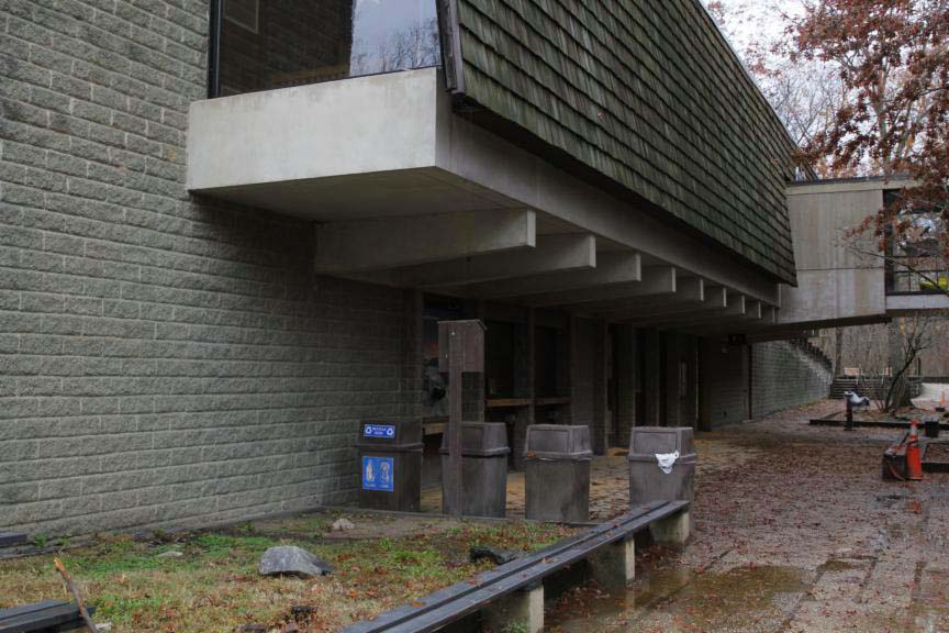
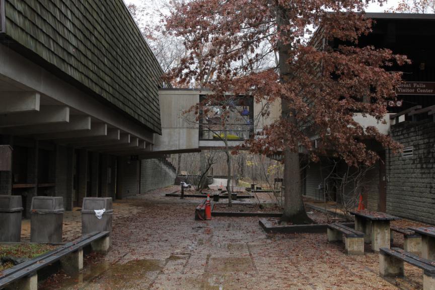
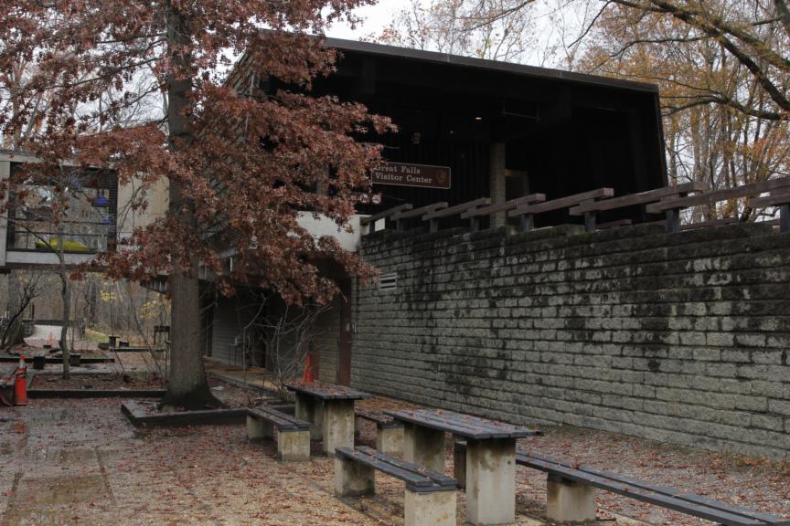
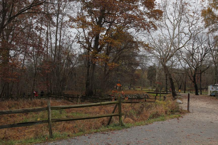
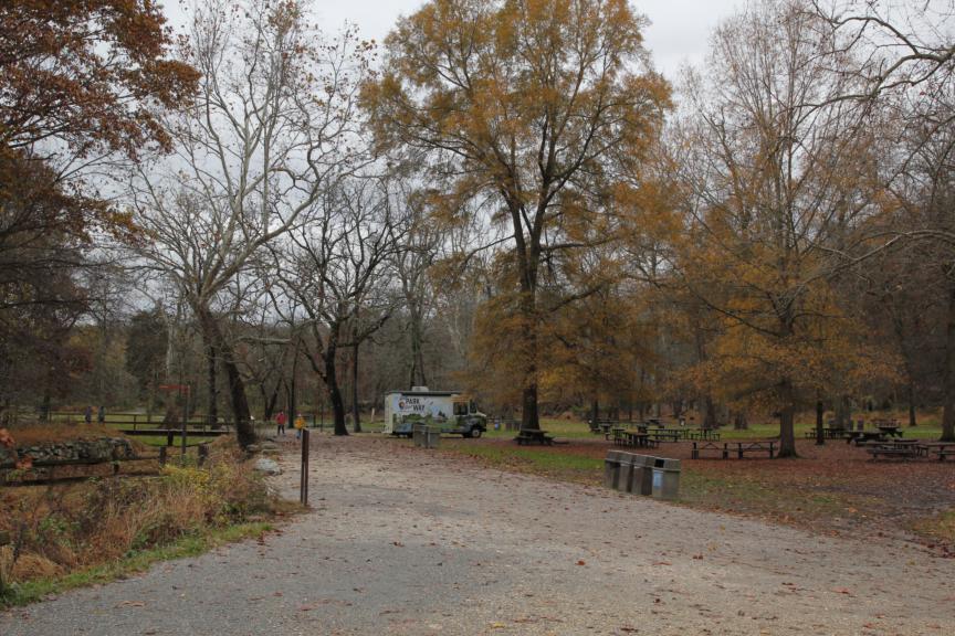
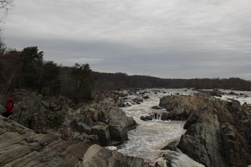
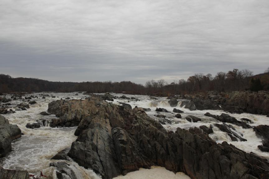
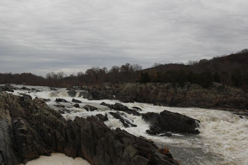
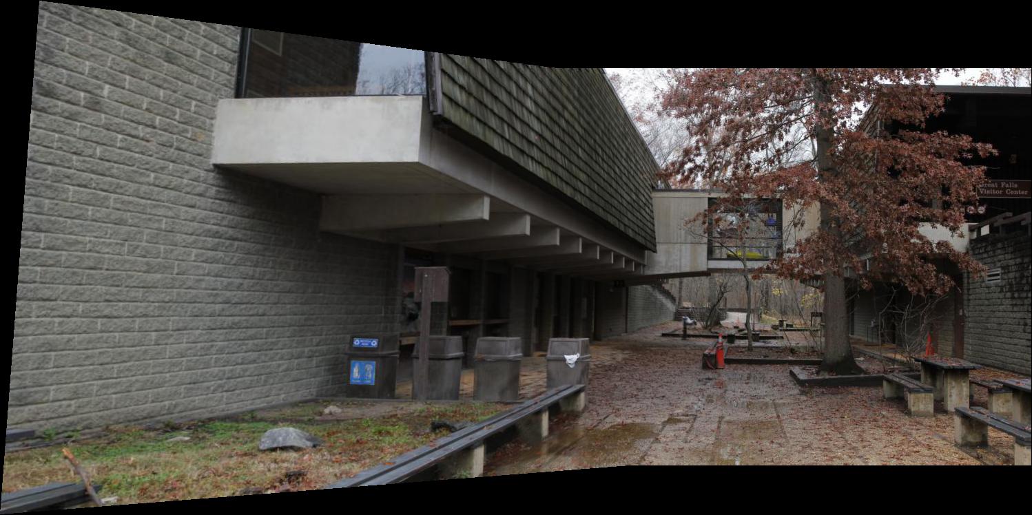
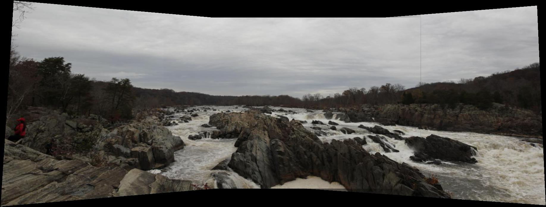
I went to the Great Fall Park, and I took three sets of photographs for this projects by simply rotating the tripod and use the Mannual Mode of camera (Canon cameras).

Before I can warp images into alignment, yI need to recover the parameters of the transformation between each pair of images. The transformation is a homography: p’=Hp, where H is a 3x3 matrix with 8 degrees of freedom. Due to the df, we actualy need 4 points for the parameters calculation, but in order to match two images perfectly, we usually choose more than 4 points. In this case, we solve the transformation with least square. And I used inverse warping for this project, so I use the inverse of the H to reconstruct the warped images.
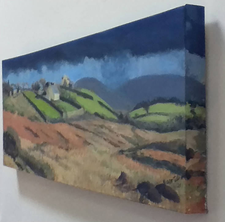
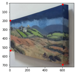
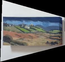
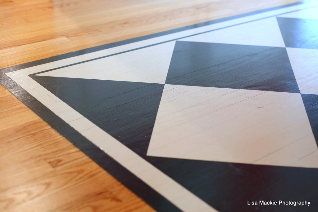
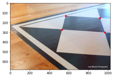
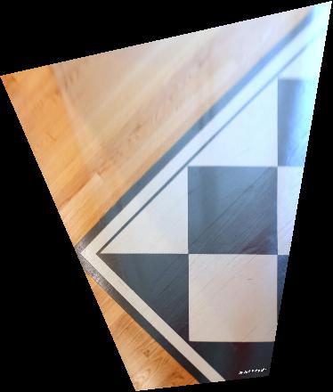
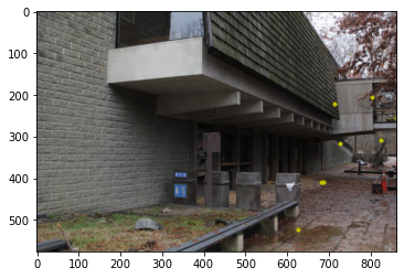
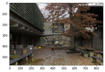
To test out my computeH and warpImage function. I chose two example images as following. And I assume that the painting on the wall is rectangular and the shape on the floor is square. Then I apply the target points and selected points to functions and get the following results.
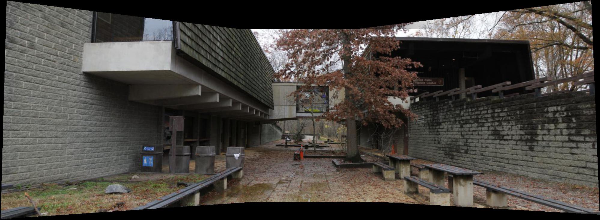
To blend images into a mosaic, I took two photos with overlapping points. I kept one image still while I warped the second image to points selected from the first. Becasue there are three photos, I first blended image on the left and the image in the middle. Then, I used the blended midway image with the right image to create the final look. I padded the image with zeros or black pixels to allow extension of the image vertically and horizontally. I have results for fixed-alpha blending.

I love this project! It is tough to finish this project and I need to think of the how to do the alpha mask since I have no experience with the mask, but I really enjoy it. And I also find out that not only the number of the points selected in the photo is important, but also the distribution of the selected point is also important. We need to let the point distributed seperately in the picture, or non-selected area will create wired stuff.
After we manually match figures in the Part A of this project. In the second part, the goal is to create a system for automatically stitching images into a mosaic. We used the same figures used in the partA. The project will consist of the following steps:
- Detecting corner features in an image
- Extracting a Feature Descriptor for each feature point
- Matching these feature descriptors between two images
- Use a robust method (RANSAC) to compute a homography
- Proceed as in the first part to produce a mosaic
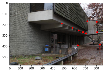
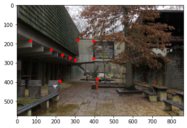
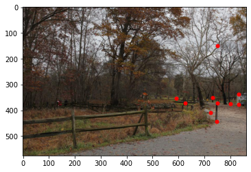
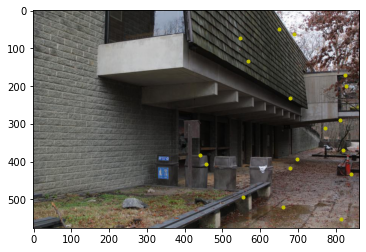
In order to automatically matching two figure, we need to find featrues that can represent each parts inside the pictures with locations. So corners of shapes is a good options. We used a Harris Interest Point Detector to find these corners in images automatically. The results of the detector on sample images from part A are shown below.
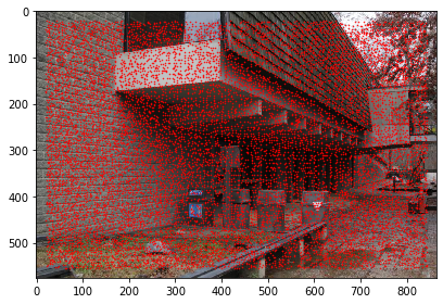
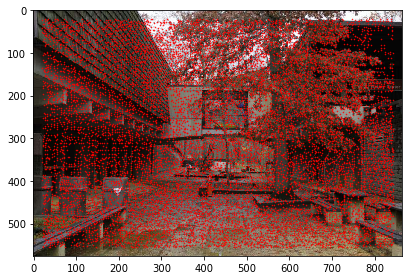
From the reuslts showing above, the number of detected corner points in the images can range up to the 10 thousands. According to Brown's paper, the best way of reducing the number of interest points is Adaptive Non-Maximal Suppression (ANMS). In ANMS, we want to restrict the maximum number of interest points extracted from each image. At the same time, it is important that interest points are spatially well distributed over the image, since for image stitching applications, the area of overlap between a pair of images may be small. This can be done by calculating the minimum suppression radius r for each point and keeping a set amount of points with the largest radius. f is the corner strength function provided by the Harris detector. Thus the minimum suppression radius r is given by

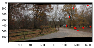
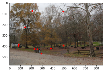
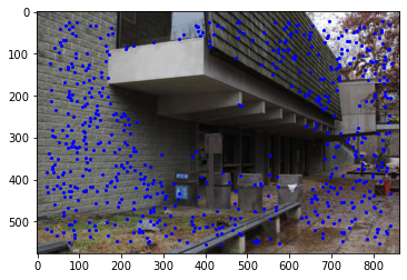
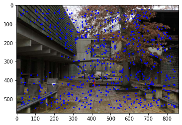
We reduce the total remian number of corners to 600. The results of the ANMS on Harris Corners results are shown below.
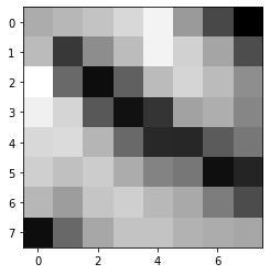
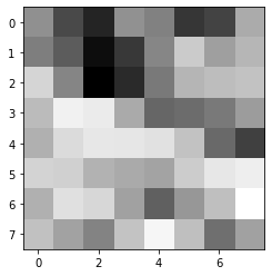
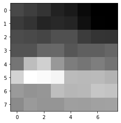
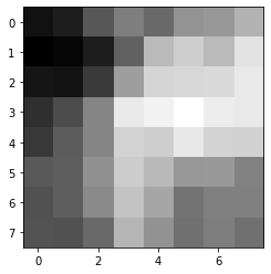
Till now we only know the location of the corners in the image, we can now use these corners to create feature descriptors. We do this by extracting a 40x40 patch centered about each point and downsampling the patch to 8x8 to eliminate high frequency signals. We also normalized the patches by subtracting the mean and dividing by the standard deviation. 5 examples of feature descriptors are shown below:

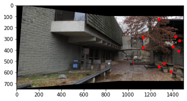
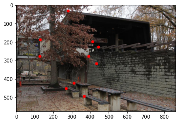
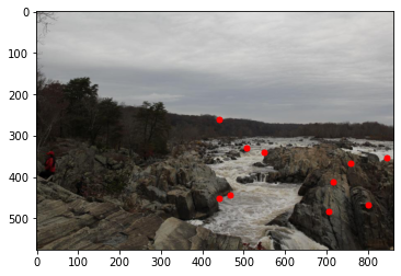
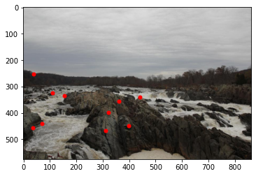
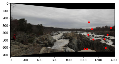
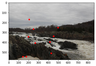
Once we have feature descriptors,we can match points together by finding the most similar patch. For each 8x8 feature in the first image, I compared it to every 8x8 patch in the second image by calculating squared distance between two patches in order to find a pair of patches that is the best match. However, not every matches are perfect. In order to find the best matches, we calculated the following values: error(1-NN) / error(2-NN), which is the ratio between the first and the second nearest neighbors. After implementing this step, our result is as follows:
Threshold: 0.3

To robustly remove bad matches in our current set of correspondences, we used random sample consensus(RANSAC). We randomly sampled 4 different point correspondences from two images, computed the homography transformation between them, calculated how many point correspondences satisfy the homography transformation below a certain threshold (here I chose 0.3 as the threhold), and finally kept the largest set of satisfied points. Our sample images have had their point correspondences reduced from 20 points to only 7 points.
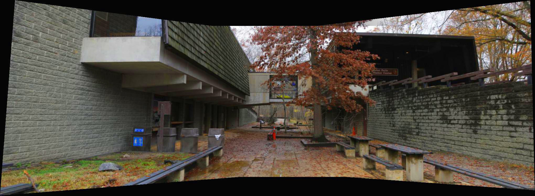
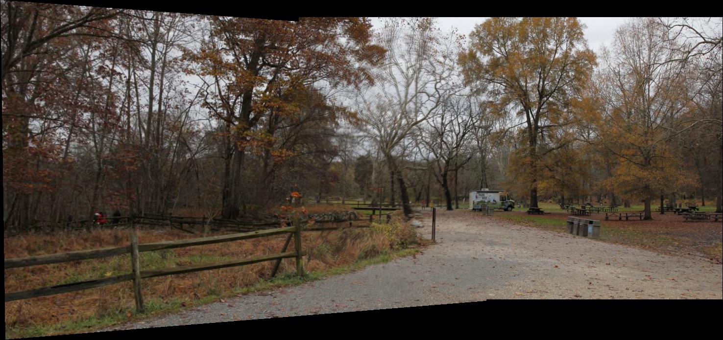
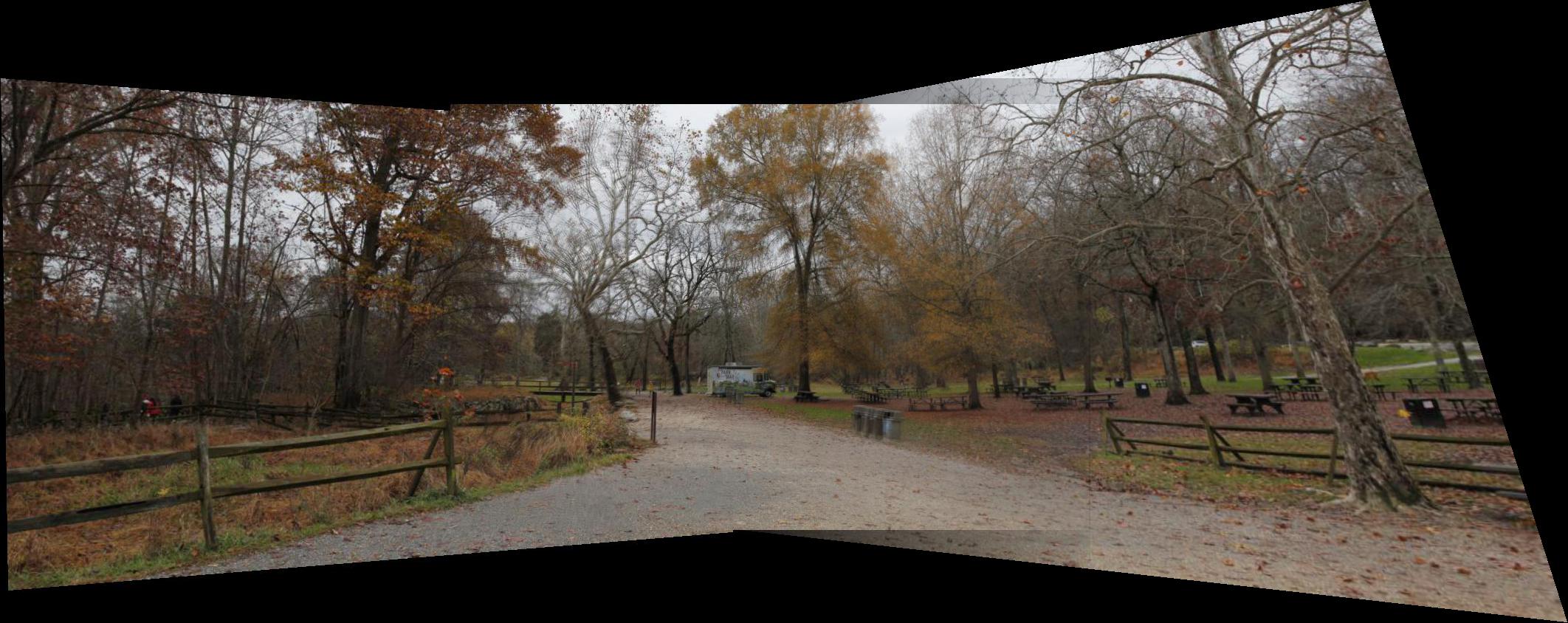
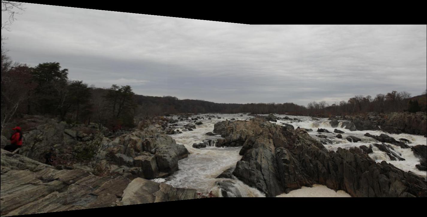
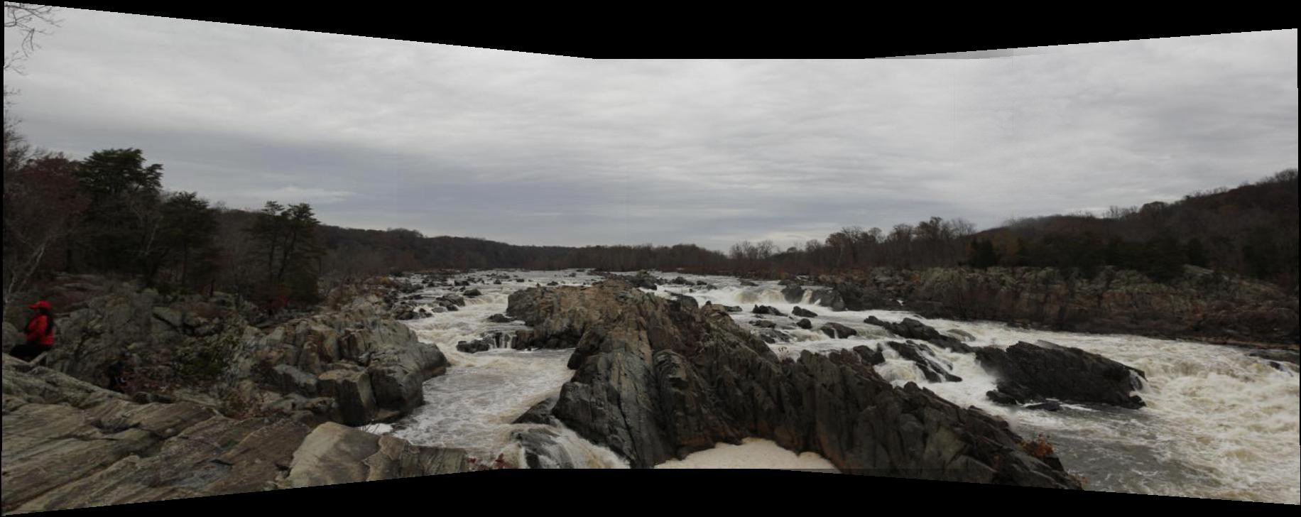
We already automaticaly find the corresponding points. Now, we can blend the images together to create mosaics. I used the same blending algorithm that was implemented in part A to produce the panoramas of three set of sample images. Same as the Part A, becasue there are three photos, I first blended image on the left and the image in the middle. Then, I used the blended midway image with the right image to create the final look. I will also compare side-by-side the manually defined correspondence mosaics from part A against the automatically produced ones.
We could see that the automatically way prodece better results. For Set 1 and Set 2, for the manually method, there are obvious blurs in the tree area, however for the automatically method, we can barely see any mismatches between two images. For Set 3, we can not find any difference between two method, which may due to the resaon that there are little trivil parts such as tree branches in the images. And also the overall color of Set 3 is dark, which make people hard to see mismtaches.

This is a biggest and toughest project for this class with a lot of complicated algorithm. I have never though of how we can use homography transformation in such many ways. More importantly, I am a photographer who do not have fancy wide-angle lens. After this project, I find myself are capable making panoramas on my own by using tripod and camera only which is exciting for me.