For this project we look at using the homography transformation for images to warp to see different perspectives in an image and then eventually use those images to blend together as a mosaic or panorama. Additionally, we also end up working with auto stiching in order to more easily do this process. Auto stiching will involve corner detection and then feature matching.
For the first part of the project, we will focus on getting images, finding the homography between corresponding points, then using that transform matrix and interpolation to warp our images. After warping to different perspectives, we will proceed to rectify images together and blend into a mosaic.
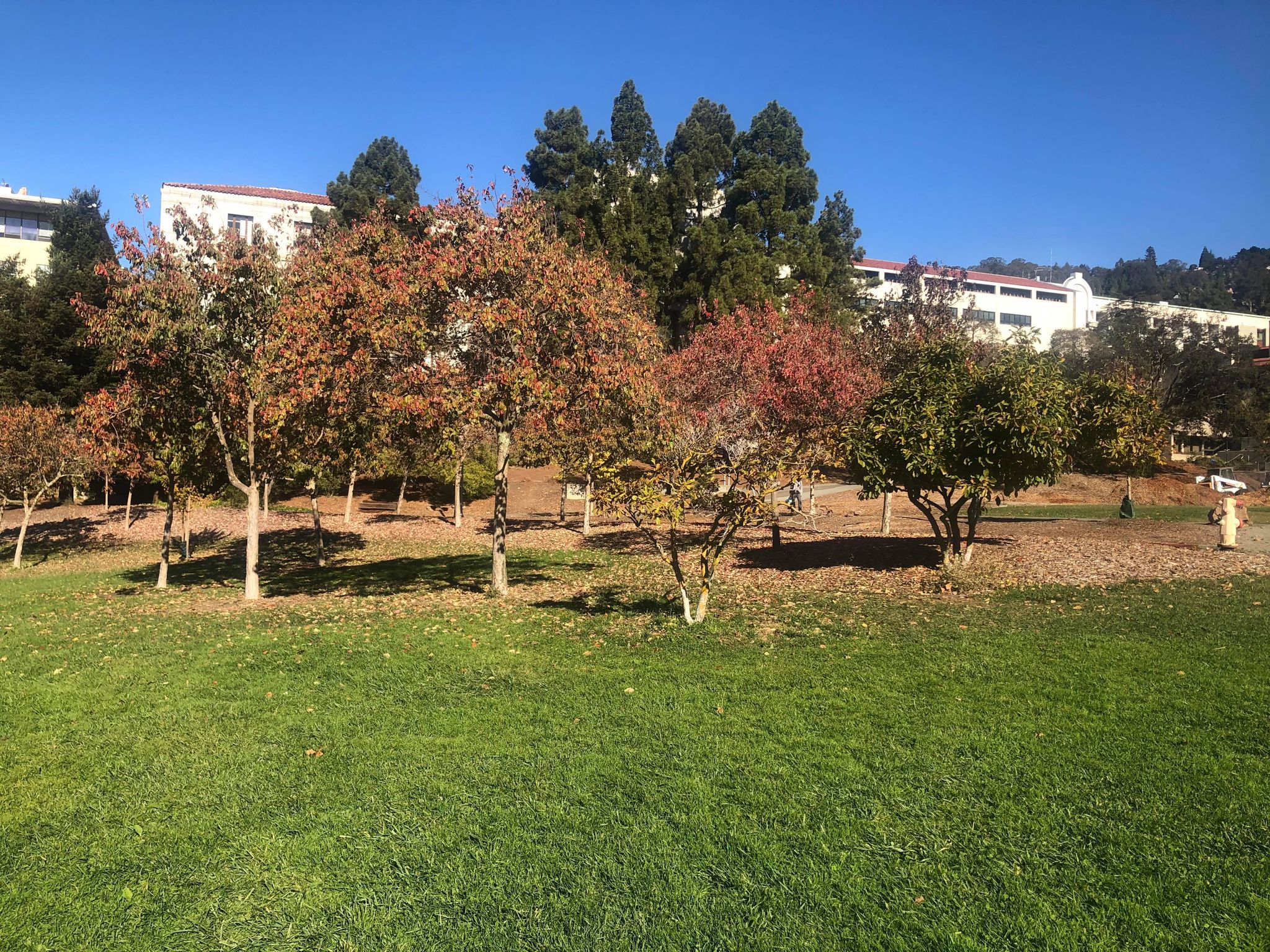
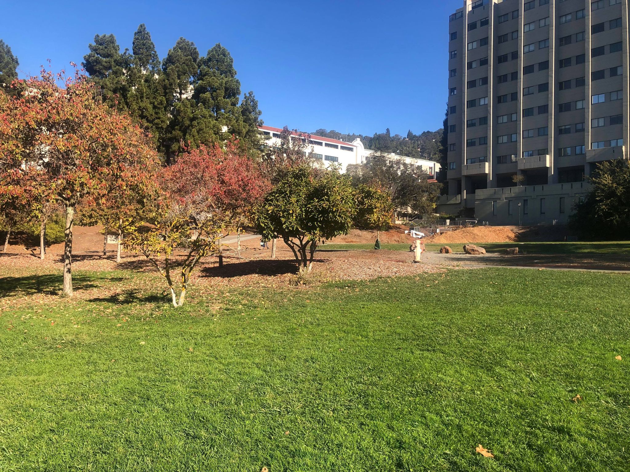
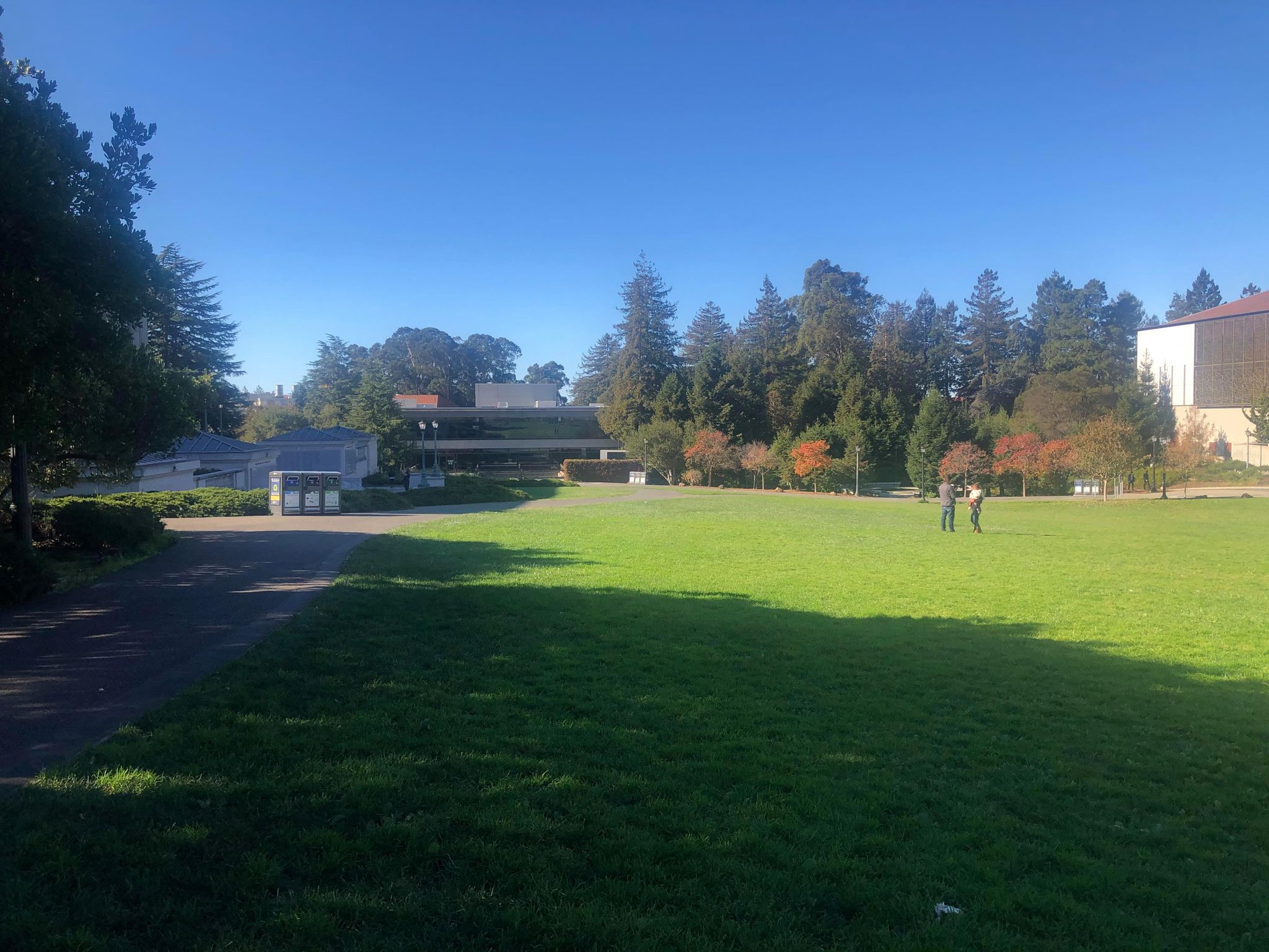
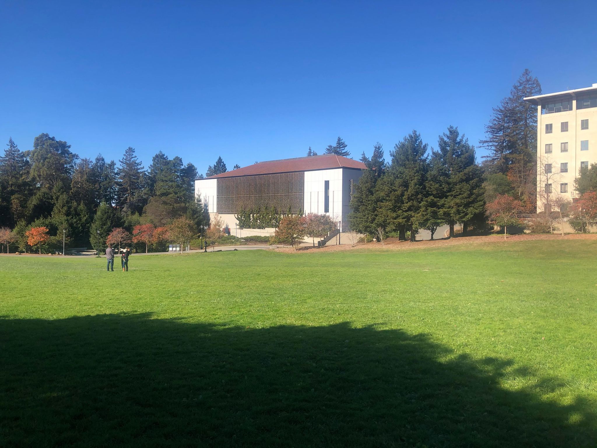
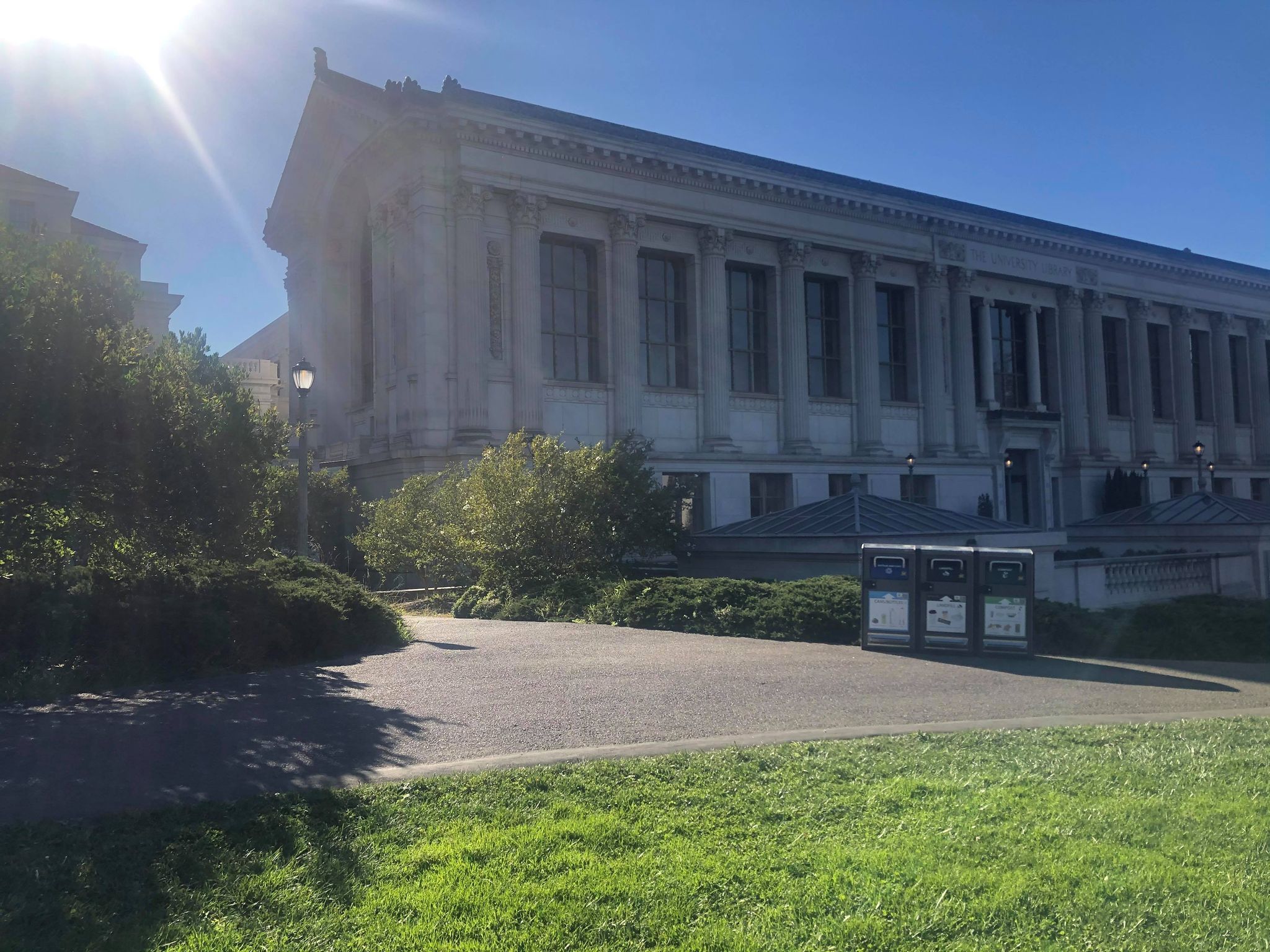
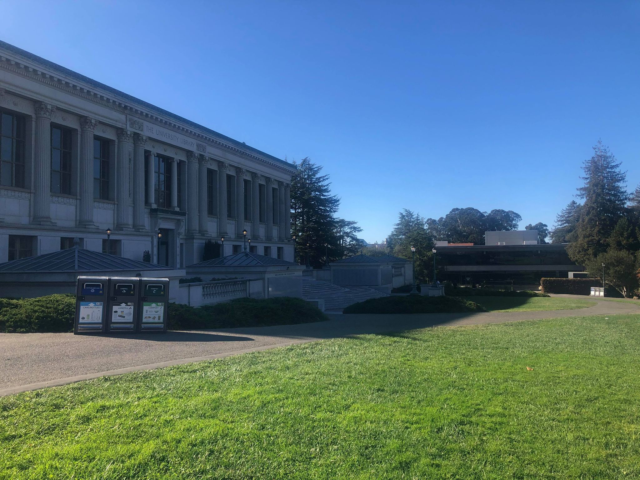
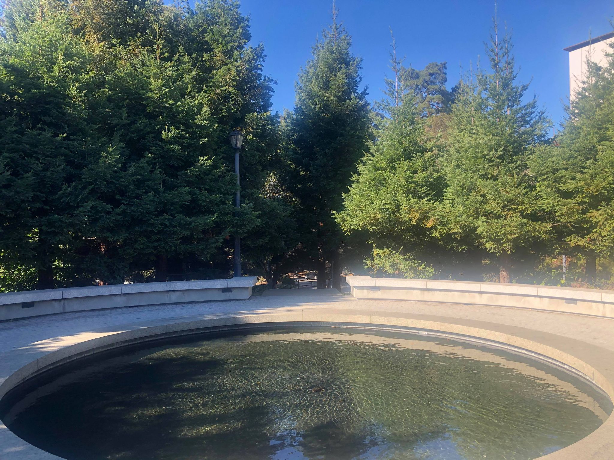
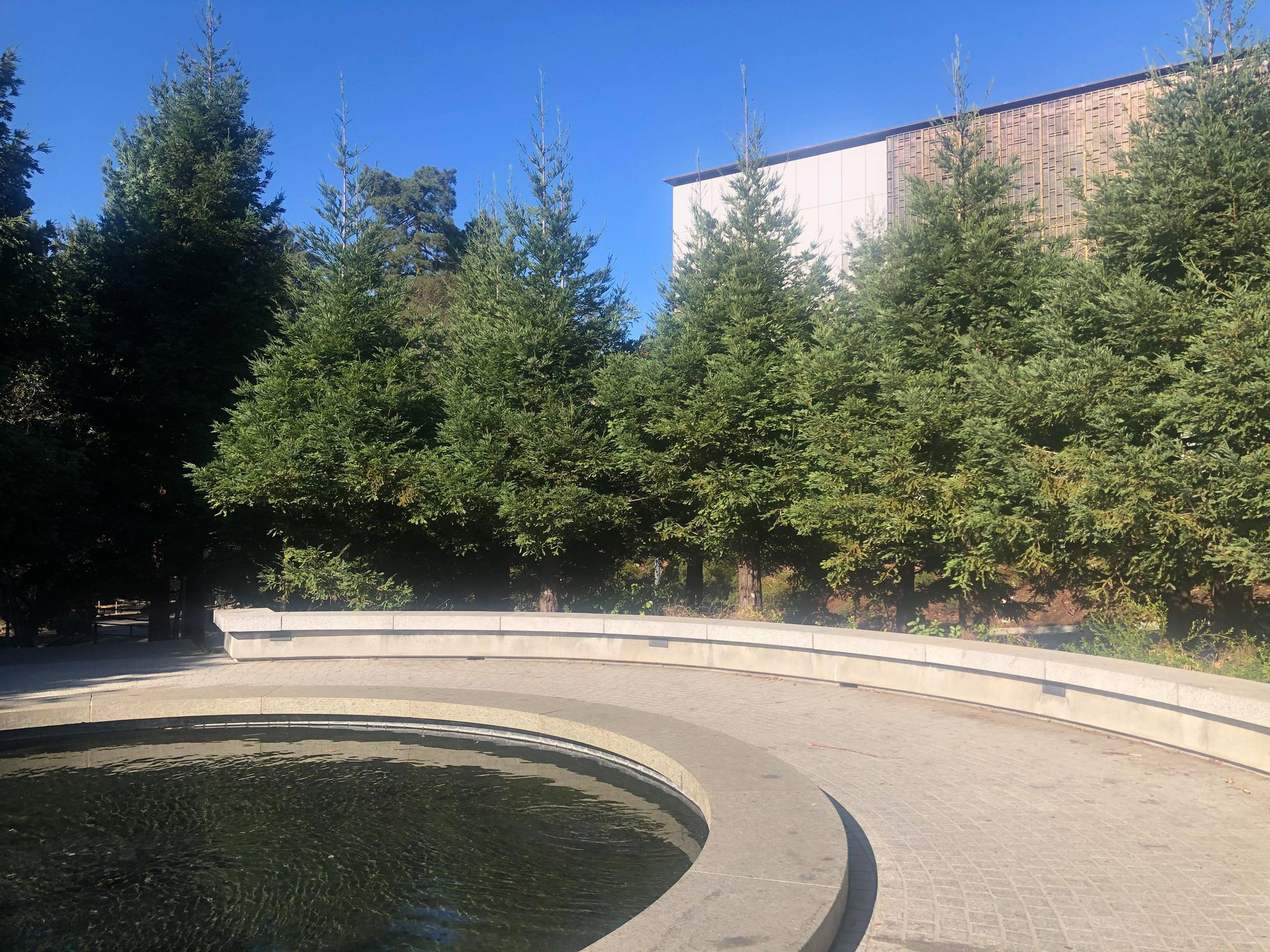
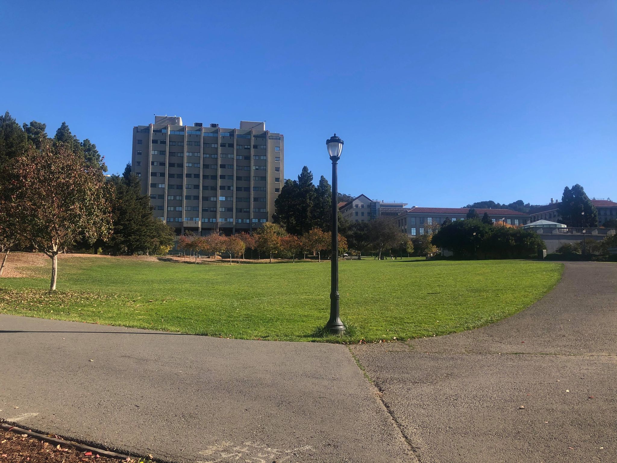
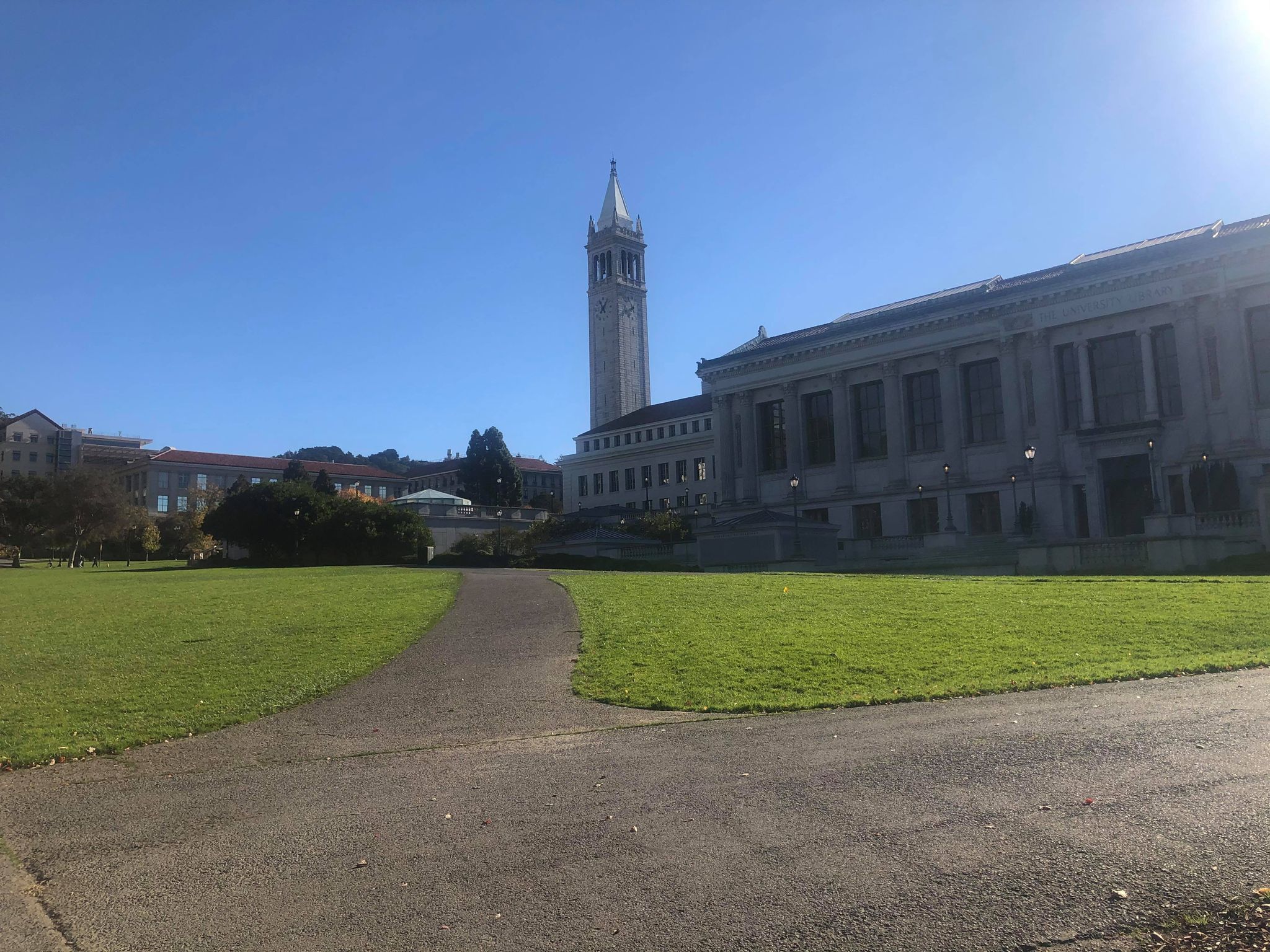
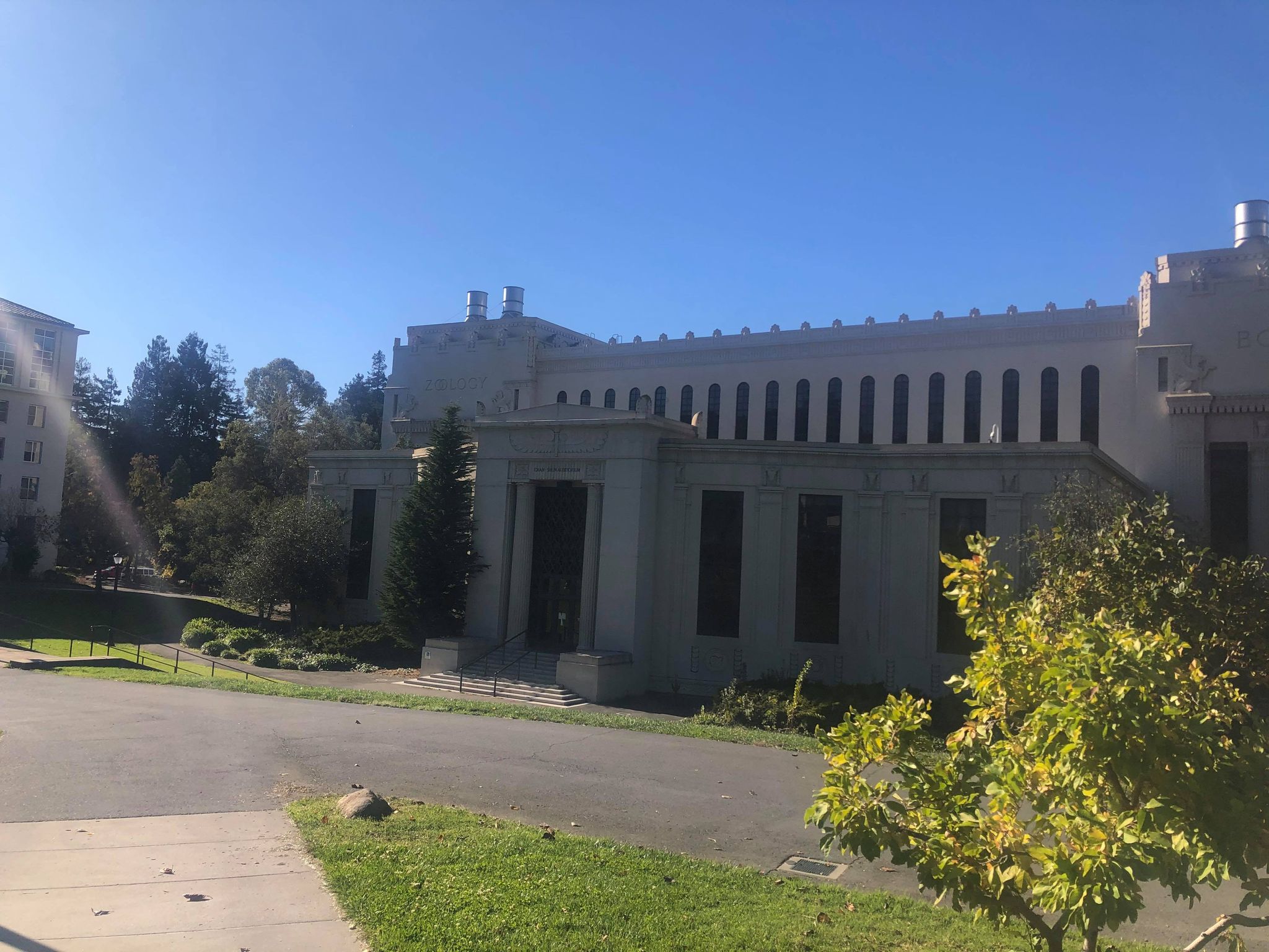
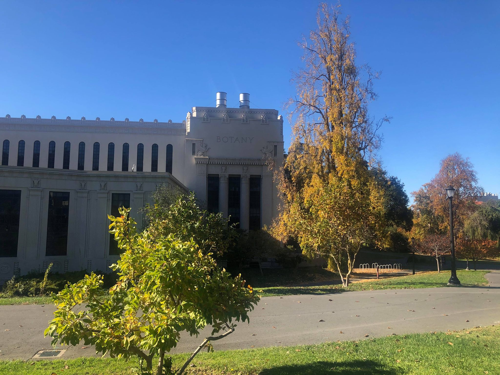
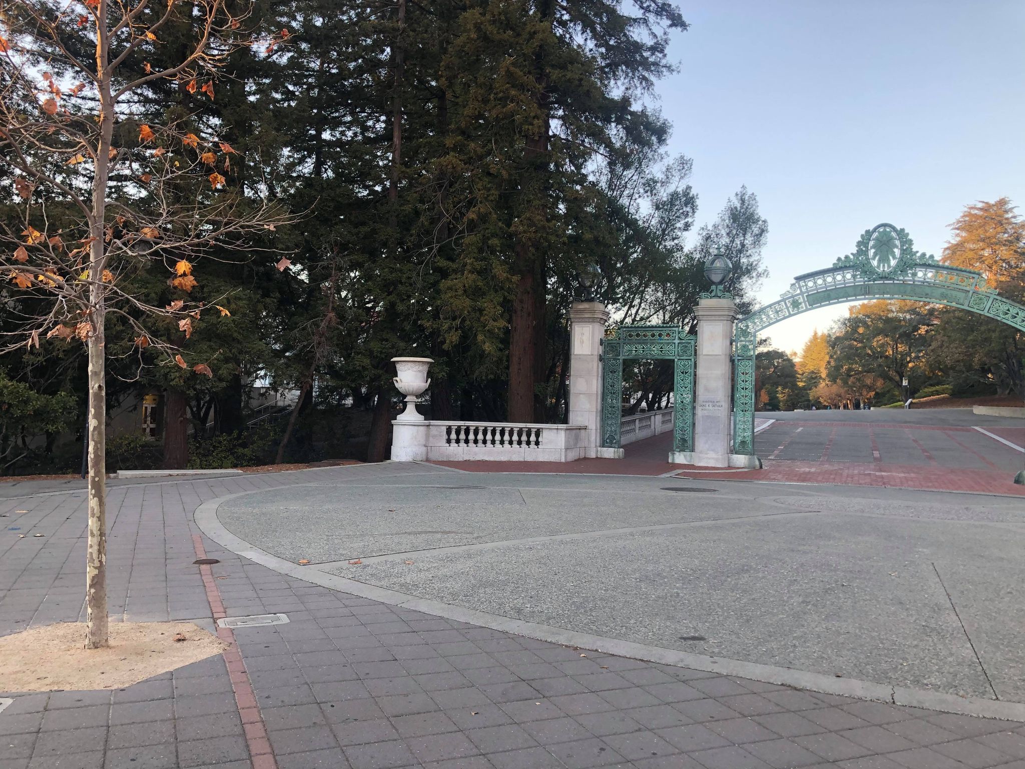
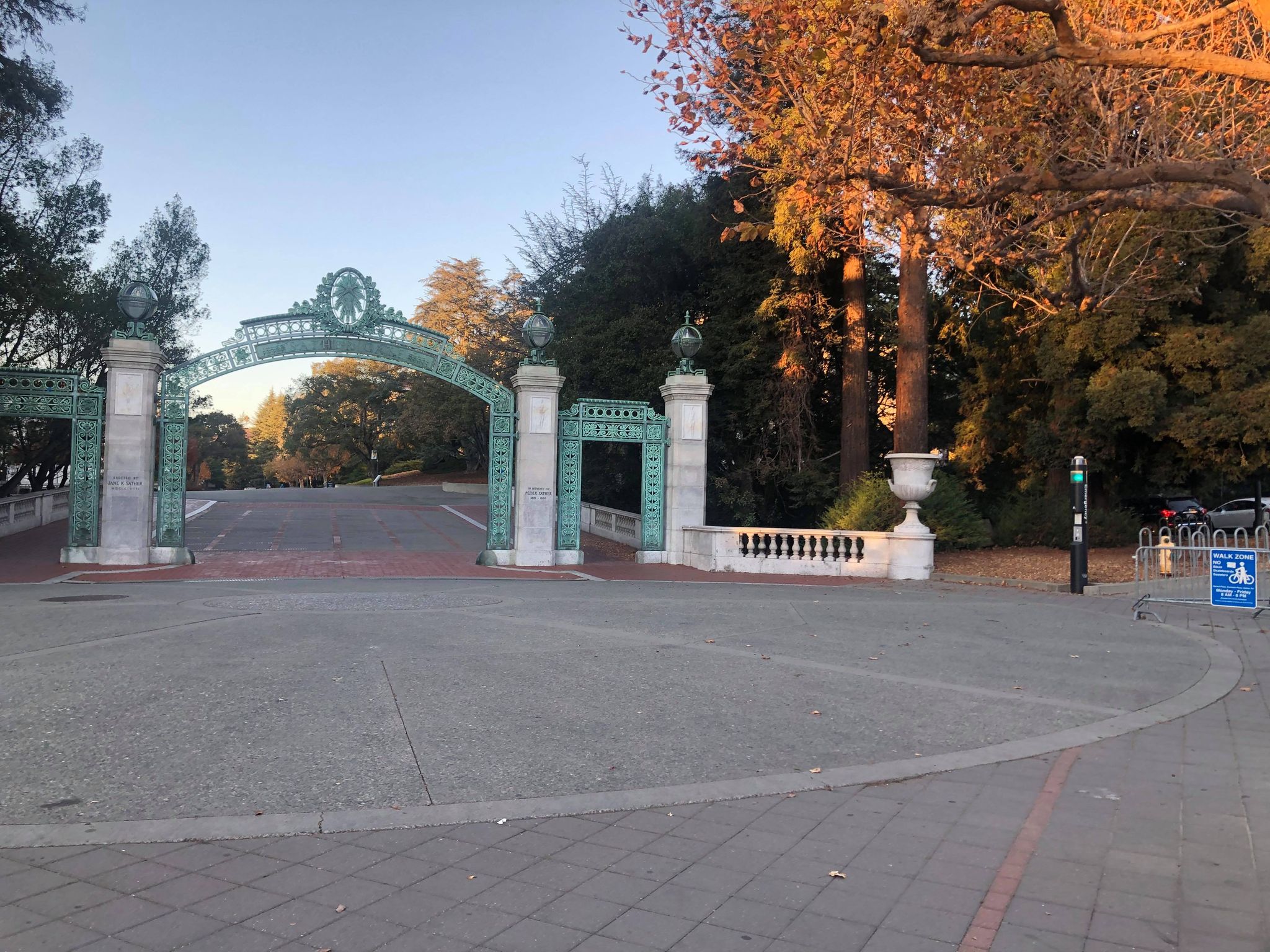
For this part, I took pictures in my studio and on campus. We want to keep the camera at the same POV, just different angles.
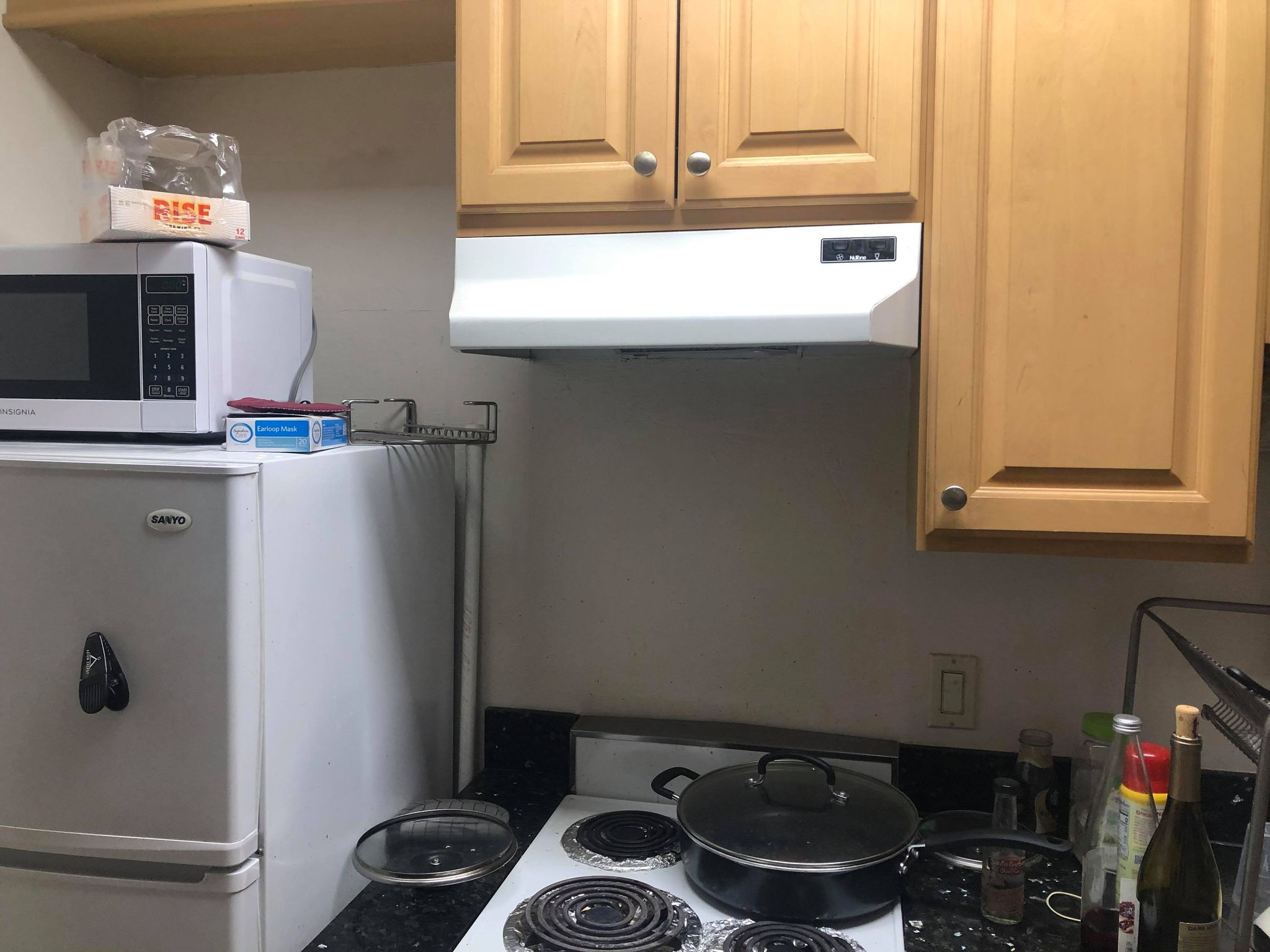
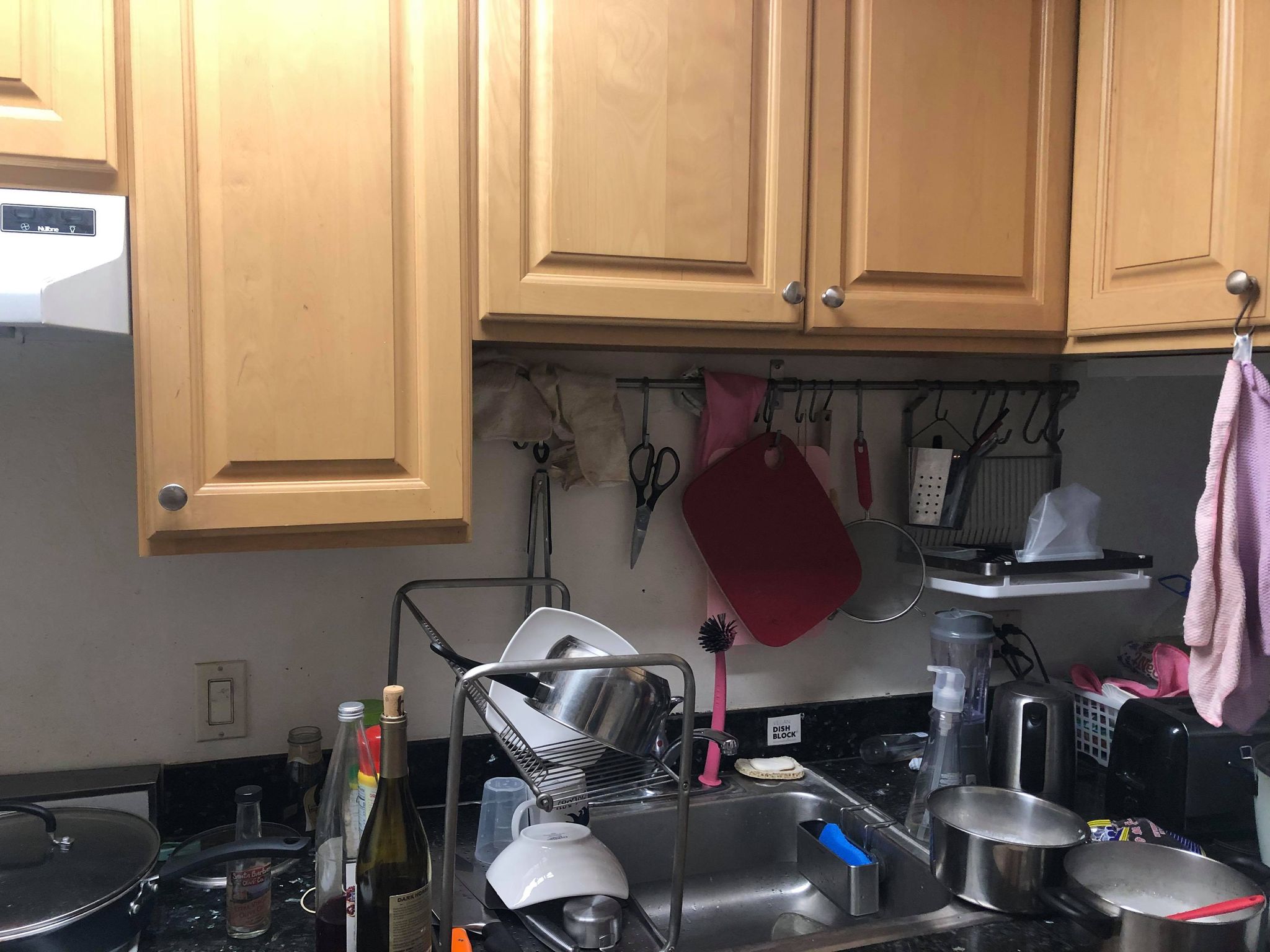
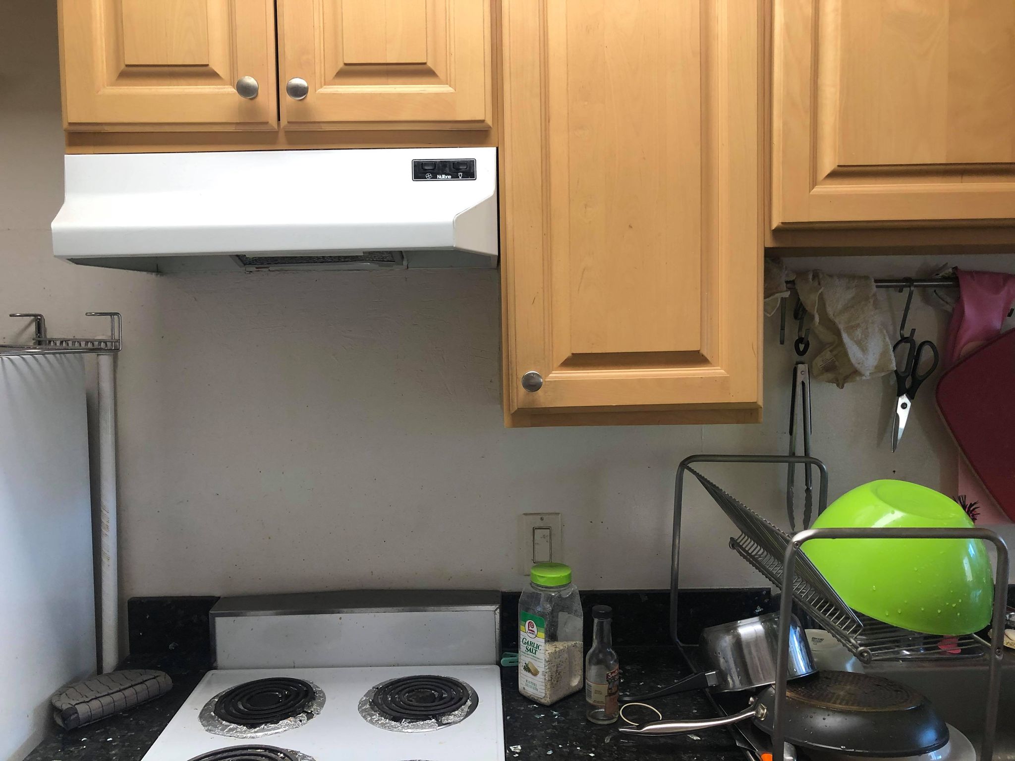
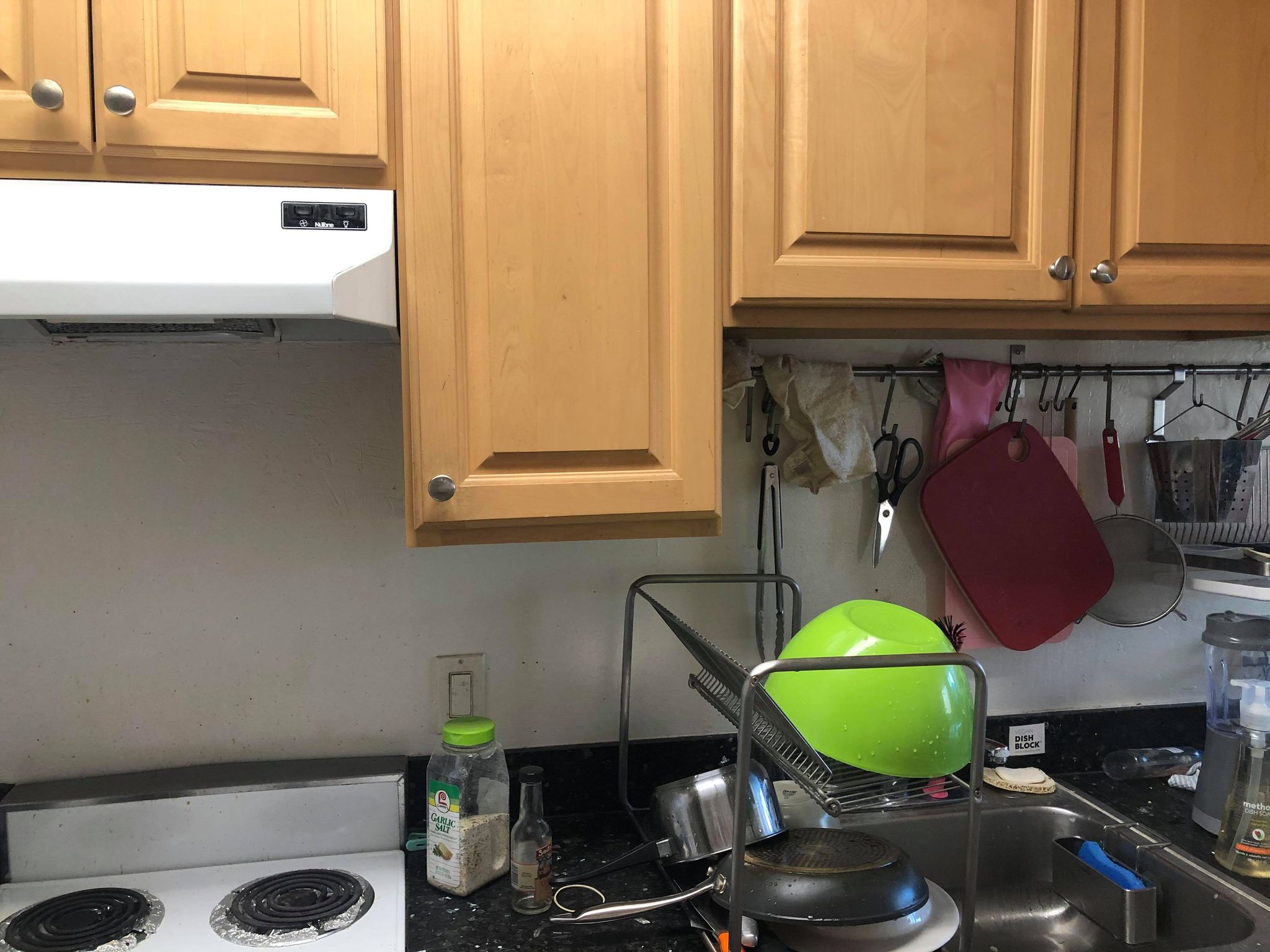
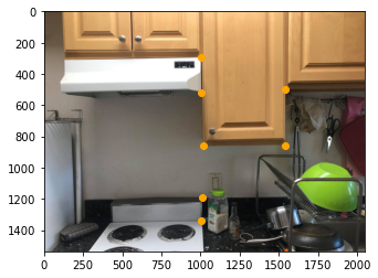
Kitchen photos
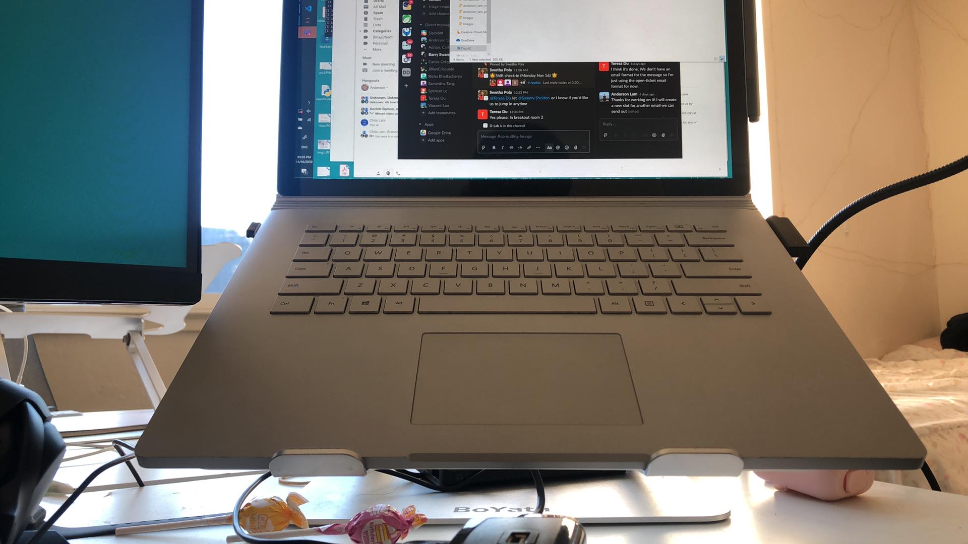
Laptop
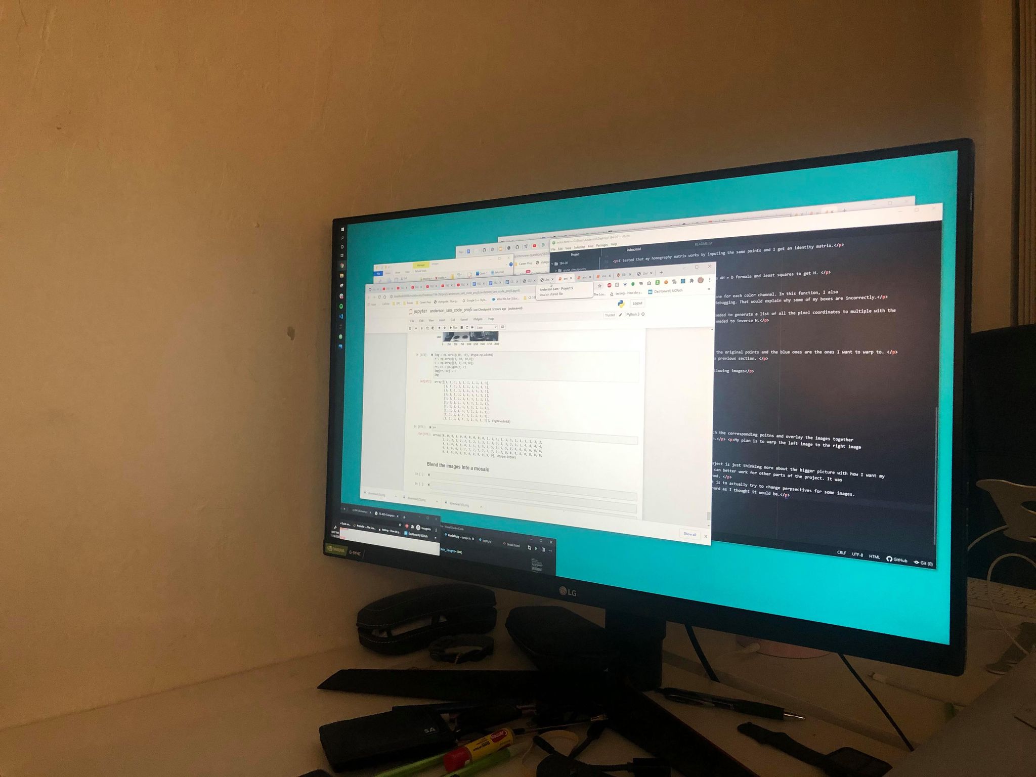
Monitor
Campus Photos
For this part of the project we utilize the AH = b formula and least squares to get H.
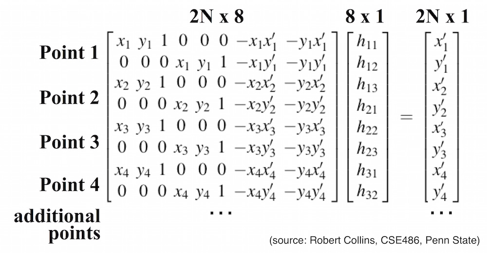
I first format my src and dst points into matrix A and then utilize least squares (np.linalg.lstsq).
I tested that my homography matrix works by inputing the same points and I got an identity matrix as warping to the same set of points, shouldn't result in any changes.
For this part of the project we utilize the AH = b formula and least squares to get H.
In this part, I used 3 interpolation functions, one for each color channel. In this function, I also generated the bounding boxes, which I am currently debugging. That would explain why some of my boxes are incorrectly.
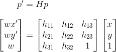
For inputs into the interpolation functions, I needed to generate a list of all the pixel coordinates to multiple with the homography matrix. I also used inverse warping and needed to inverse H.
For these photos, the orange points are the new points to fix to.
.png)
.png)
.png)
.png)
.png)
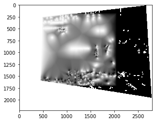
This part utilize the same function warp from the previous section. However, I needed to do some modifications to add some sort of offset.
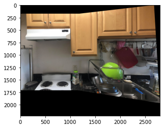
I warp the image on the right to the left image.
.png)
.png)
For this part I will be using translation to match the corresponding poitns and overlay the images together for a mosaic from the images in the previous section.
I already have a warped right image to left image from the previous part. For this part, all I needed to do more was to create another image with the correct offsets so that they would align correctly.
Afterwards, I needed to create a blend layer to correctly blend the colors together. I ended up using the moprh distance transform function in order to determine the image distances from each other.
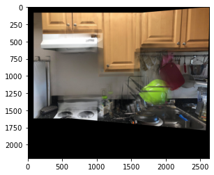
The image to the left is the left image inside the warped image dimension with the appropriate offsets. Then, it is the mask I applied, resulting in the final combined image in the right.
.png)
Failure with misalignment example (incorrect offsets)
Below are the points that I selected for both image
.png)
.png)
.png)
.png)
.png)
.png)
Below are the points that I selected for both image
.png)
.png)
.png)
.png)
.png)
.png)
Below are the points that I selected for both image
.png)
.png)
.png)
.png)
.png)
.png)
The most important thing I learned about this project is just thinking more about the bigger picture with how I want my data to be and how I want to to be formulated so it can better work for other parts of the project. It was also very important with how my points were determined.
The coolest thing I learned is simply how easy it is to actually try to change perpsectives for some images. Computing the H matrix and applying warp wasn't as hard as I thought it would be.
Now that we created a blending solution, the next step is to grab the points automatically so that we can more quicky gather correct corresponding points to stitch together. The points we will grab are corners as they are best compared to edges and other points as they are easier to detect with that way corners are formed. Then, we will filter down the best points, then create feature descriptors from those. The feature descriptors will make it easy for us to compare and match features together. Aftwards, we want to find out the corresponding points with RANSAC.
For this section, I used the sample code given by Prof Efros. However with the basic code, it took my computer to run anms, a very long time since I got thousands of points. To correct this, I used the corner_peaks function instead and made the min distance in corner_peaks to be editable.
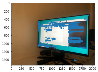
This is an example of running the corner detection on my monitor and campus.
.png)
.png)
For this section, I create a new list to later return after finding the best points. To do this, I do a loop on a point for all the points and I basically have an algorithm to reach some threshold and I continue to update some "R" value as given in the ANMS Function.
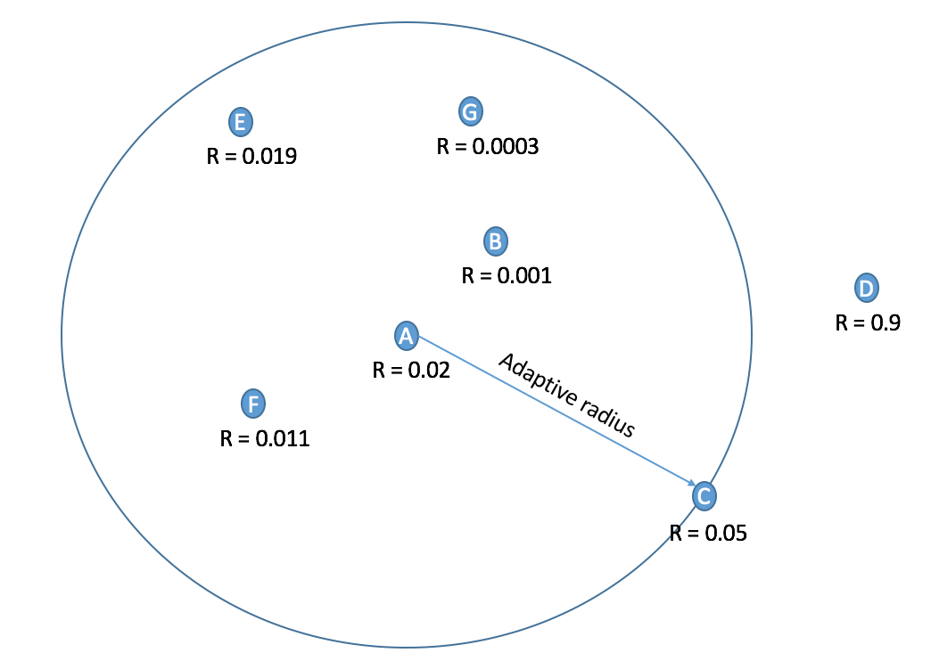
At the end of the loops, get the values that have the best R values respectively.
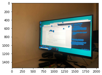
This is an example of running ANMS, to reduce the number of points from harris.
.png)
.png)
The algorithm for this part is relatively simple. We want to get the patch of every point we kept from ANMS. To do this, we create a list to store the values and loop through all of the points we have and then get the patch in a 40x40 box (or 20 pixel raidus) and then downsize it to a (8x8 radius) and normalize it. Normalization is done by subtracting it from its mean then dividing by its std.
Here are examples of some feature descriptors.
.png)
.png)
.png)
.png)
For feature matching, we determine which detected points are together. This is done by using the supplied dist2 function given from Prof Efros as well as the feature descriptors. To do this, I made loop of every feature descriptor in image1 for every feature descriptor in image2. This is so we can compare every feature descriptor together. To better compare them, I flatten the feature descriptors by reshapring the 8x8 feature descriptors into 1x64. At the end I calculate the distance using the dist2 function. Based on those distances, we will be able to determine whether or not two feature descriptors or points are together or not.
.png)
.png)
For the RANSAC (Random sample consensus) algorithm, we basically select 4 feature pairs at random, compute the homography, compute inliers and keep the
largest set of inliers. To do this, I had 2 loops. One for a give number of iterations, another for the all points in my matches.
From there, I get points from image1 and warp the points from image2 to image1 using the homography I computed. Based on the
predicted and actual points, I will then compute SSD to determine whether or not to keep the inliers.
SSD: sum of (actualPair - predictPair)^2
Below are the final points that RANSAC determined to be best together.
.png)
.png)
.png)
.png)
In this section, I simply combined all of the functions from the previous parts into a quick an easy function that generates the correct H and gets the correct points.
.png)
.png)
.png)
.png)
.png)
.png)
.png)
.png)
.png)
.png)
.png)
.png)
In comparison, the autostitching almost always out performs the manual stitching. I had some problems with some of the images manually stitching, but auto was able to get precise points.
.png)
.png)
.png)
.png)
.png)
.png)
.png)
.png)
.png)
.png)
.png)
.png)
For this part, I tried to do the panormaic matchings (given an unordered set of images) as mentioned in this paper: http://matthewalunbrown.com/papers/iccv2003.pdf
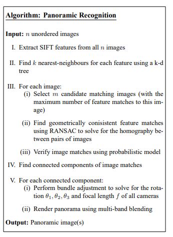
I first created a function to load in all the images and return a dictioanry to the file loaded. After, I created a function, getAllANMS, to return a dictionary from the image name to the ANMS points. After that, I ran an algorithm to determine if there is a pairing for all images. (double nested for loop to try to pair each one). Based on some threshold, I determine if it is a pair or not. The loops for determining pairings is the longest running algorithm. It might have been better to run on a smaller sample or utilize the kNearest algorithm described. I did not go about that method as it seemed more complicated than necessary. Lastly, based on those pairings, I will then compute the H for all the pairings. I return a dictionary of pairings of file names and their homography matrix and respective points. From these resulting_pairs, I can then use my function blend() to automatically blend the images together.
I have implemented this algorithm in my code at the very bottom.
The computation for the homography is calculated from the RANSAC function I derived earlier.
Completing this proejct was really satisfying, as I had just completed autostitching with efficient math and code. This project was challenging for me though, in calculating the correct warp shapes to pair together as well as creating a blend. I learned more about how photos work and how powerful the homography transformation is. The concept of the feature descriptor is also interesting to utilize and I wonder what other applications of it is possible.